E.C Classic ML Roadmap

Use this elective when your dataset is small, your features are clear, or you need a strong baseline before trying a heavier model.

See the Baseline Map First

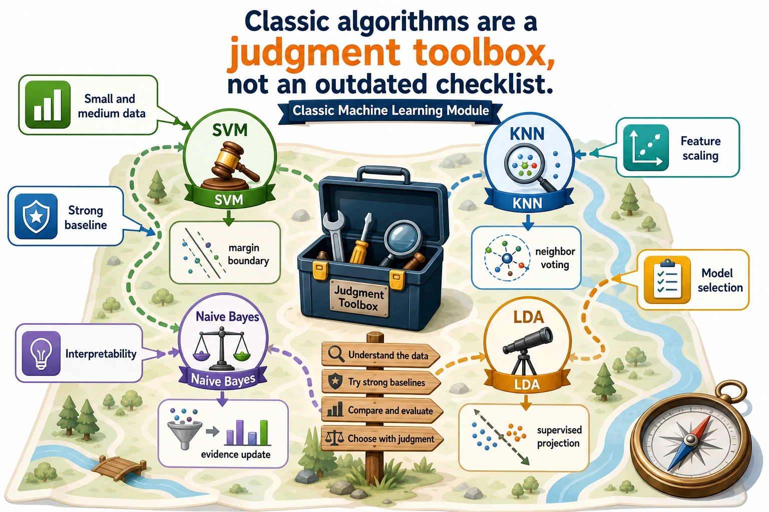
Classic ML helps you answer: is the problem already solvable with simple features?

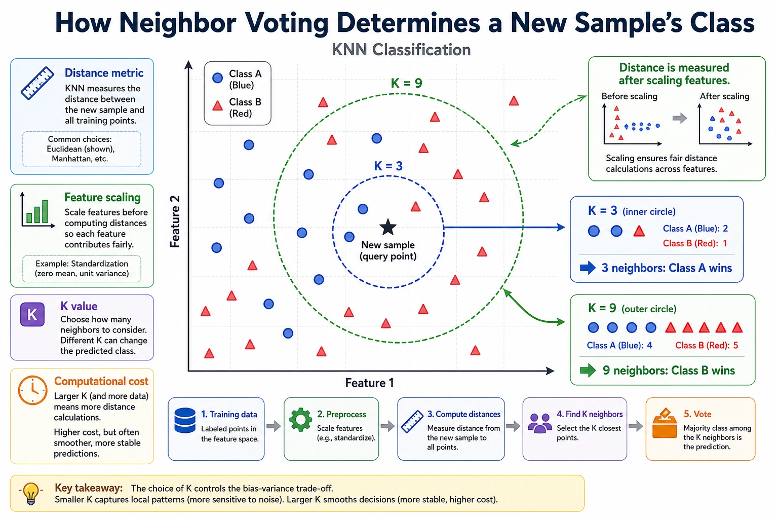
Run the Smallest KNN Baseline

def distance(a, b):
    return sum((x - y) ** 2 for x, y in zip(a, b)) ** 0.5

train = [
    ([0.1, 0.2], "low"),
    ([0.2, 0.1], "low"),
    ([0.8, 0.9], "high"),
    ([0.9, 0.8], "high"),
]

point = [0.75, 0.85]
nearest = min(train, key=lambda row: distance(row[0], point))
print("prediction:", nearest[1])
print("neighbor:", nearest[0])

Expected output:

prediction: high
neighbor: [0.8, 0.9]

This is the smallest baseline habit: define features, compare distance, predict, and keep the result for later comparison.

How To Use This Module In A Real Project

Use classic ML as a baseline contract. Before reaching for a larger model, ask whether clear features and a simple decision rule already solve enough of the problem. If the baseline is strong, the heavier model must justify its extra cost.

The best evidence is comparative: same split, same metric, and one limitation note. For example, “KNN is readable and fast to build, but prediction cost grows with stored examples,” or “Naive Bayes is cheap for ticket routing, but it misses wording that depends on context.”

Learn in This Order

Step	Lesson	Practice Output
1	E.C.1 SVM	Explain margin, support vectors, C, and kernel choice
2	E.C.2 KNN	Build a distance-voting baseline
3	E.C.3 Naive Bayes	Convert evidence counts into class probabilities
4	E.C.4 LDA	Project features to separate classes

How To Use This Module In A Real Project

Use classic ML as a baseline contract. Before trying a larger model, ask whether clean features plus SVM, KNN, Naive Bayes, or LDA already solve most of the task. If the baseline is strong, the larger model must justify its extra cost.

Keep the comparison concrete: same train/test split, same metric, and at least one failure case. This turns classic ML from a theory detour into a practical guardrail against overbuilding.

Evidence to Keep

Keep this page’s proof of learning as a small evidence card:

Model Family

SVM, KNN, Naive Bayes, LDA, or another classical baseline

Dataset View

feature scale, class balance, decision boundary, and train/test split

Metric

accuracy/F1, confusion matrix, margin, neighbor behavior, or projection quality

Failure Check

scaling, high dimensionality, weak assumptions, leakage, or poor baseline fit

Expected Output

classical-ML baseline result with one limitation note

Pass Check

You pass this module when you can build one classic baseline, explain why it is appropriate, and compare it with a heavier model or later project result.

Check reasoning and explanation

A solid baseline answer names the dataset shape, model family, and comparison point. For example: “KNN is acceptable here because the dataset is small and distances are meaningful; I will compare it against a later neural model using the same split and F1 score.”

The answer is incomplete if it only reports accuracy. Classic ML is most useful when it gives a fast, interpretable reference and a clear limitation, such as feature scaling, nonlinear boundaries, or high-dimensional sparsity.