6 Deep Learning and Transformer Basics

Chapter 6 has one job: help you understand how a model learns from loss, gradients, and repeated training steps.

Where You Are In The Main Route

You have already trained sklearn models and judged them with metrics and error samples. This chapter opens the training loop: tensors carry data, a model produces predictions, loss measures error, backpropagation computes gradients, and the optimizer updates parameters.

This is the last model-foundation chapter before LLMs. The goal is not to master every architecture before moving on. The goal is to understand training, shapes, attention, and Transformer blocks well enough that Chapter 7 no longer feels like magic.

See The Training Loop

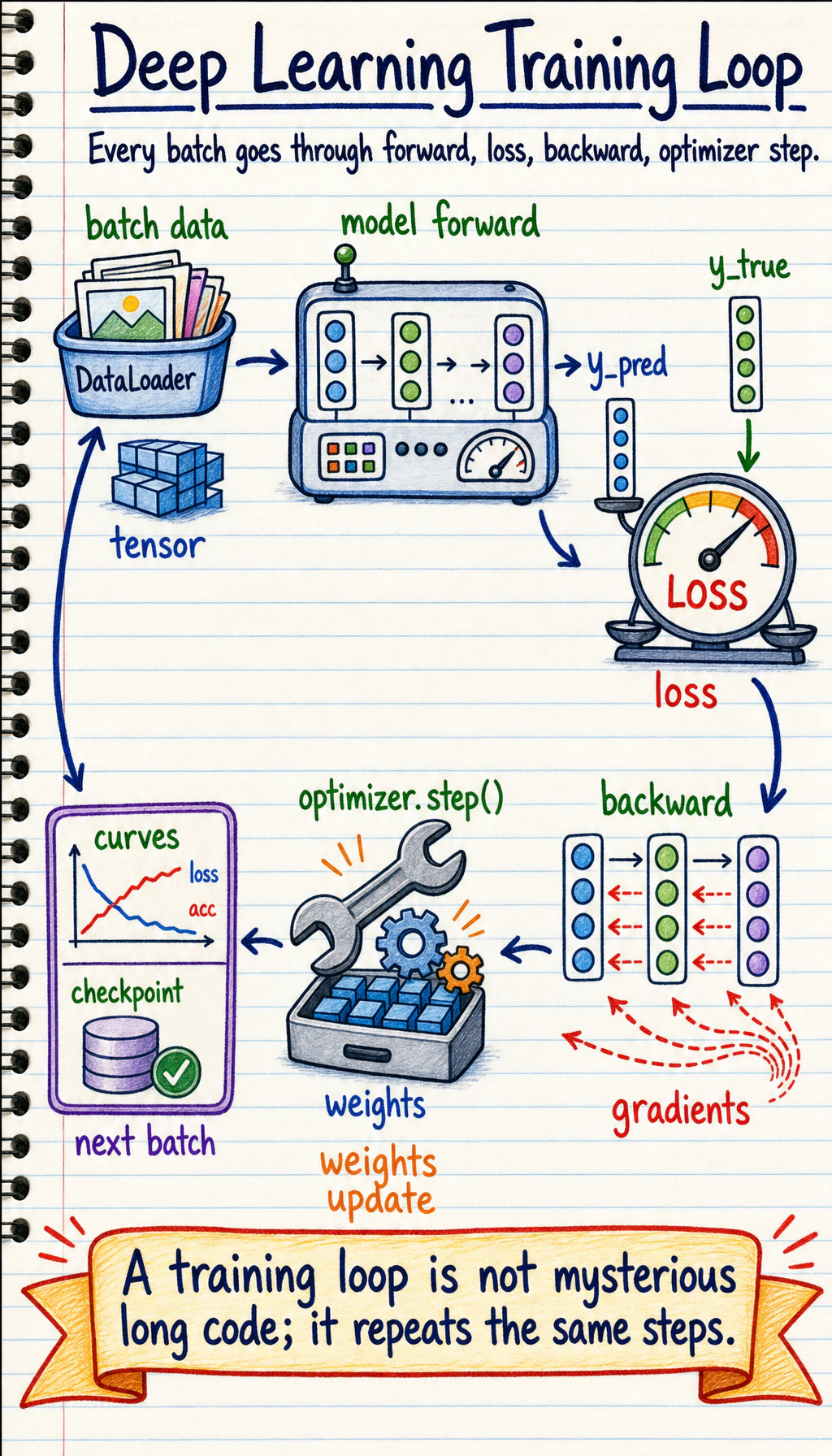
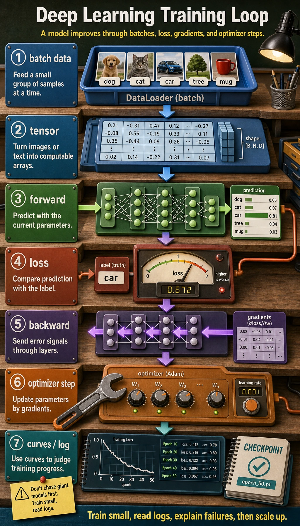
Read the picture first. Most deep learning training code is this loop:

batch data→model forward→loss→backward gradients→optimizer step→curves

Do not start by chasing large models. First make a small model train, log what happened, and explain why it improved or failed.

Learning Order And Task List

Use this checklist as both the chapter guide and the task sheet. Follow the core path first: 6.1 -> 6.2 -> 6.5 -> 6.8. Treat CNN, RNN, generative models, and training tips as extensions you return to when a project needs them.

1. 6.1 Neural Network Basics Follow along: understand neurons, activations, forward/backward pass, optimizers, regularization, and initialization. Evidence to keep: one hand-written training-loop explanation.

2. 6.2 PyTorch Follow along: practice tensors, autograd, nn.Module, Dataset, DataLoader, and a minimal training loop. Evidence to keep: one runnable PyTorch script.

3. 6.5 Transformer Follow along: learn Query, Key, Value, self-attention, positional encoding, and Transformer blocks. Evidence to keep: one attention input/output diagram.

4. 6.8 Projects and 6.8.5 Workshop Follow along: build a PyTorch evidence pack before larger image, sentiment, or generative projects. Evidence to keep: logs, curves, checkpoint, shape trace, and README.

5. 6.3 CNN Follow along: use image classification to connect data shape, convolution, pooling, and transfer learning. Evidence to keep: shape notes and one image-classification run.

6. 6.4 RNN Follow along: learn why sequence data needs memory and how LSTM/GRU helped before Transformer. Evidence to keep: one sequence-model note.

7. 6.1.8 Optional DL History Follow along: skim why backprop, CNN, RNN, Attention, and Transformer appeared after you know the main loop. Evidence to keep: a short “why this architecture exists” note.

8. 6.6 Generative Models and 6.7 Training Tips Follow along: treat as extensions after the training loop is stable. Evidence to keep: one tuning or diagnosis note.

Core Path, Extensions, And Depth

Layer	What to study now	How to use it
Required core	Tensor shape, autograd, nn.Module, Dataset/DataLoader, training loop, validation curve, Attention, Transformer	These become the mental model for tokens, context, and LLM behavior in Chapter 7
Optional extension	CNN, RNN, GAN/VAE, compression, advanced tuning	Return here when an image, sequence, generative, or deployment project needs the extra depth
Depth challenge	Overfit one tiny batch on purpose, then explain what that proves and what it does not prove	This makes later training failures easier to debug

Key terms for this chapter:

Term	Meaning
tensor	Multi-dimensional array used by PyTorch
forward	Data passes through the model to produce predictions
loss	Number that measures prediction error
backward	Computes gradients from the loss
optimizer	Updates parameters using gradients
epoch	One pass through the training data
batch	A small group of samples processed together

First Runnable Loop

Install PyTorch from the official selector if needed, then run this tiny loop after PyTorch is available:

import torch
from torch import nn

torch.manual_seed(42)
x = torch.tensor([[0.0], [1.0], [2.0], [3.0]])
y = torch.tensor([[0.0], [2.0], [4.0], [6.0]])

model = nn.Linear(1, 1)
loss_fn = nn.MSELoss()
optimizer = torch.optim.SGD(model.parameters(), lr=0.1)

for epoch in range(20):
    pred = model(x)
    loss = loss_fn(pred, y)
    optimizer.zero_grad()
    loss.backward()
    optimizer.step()
    if epoch in {0, 1, 5, 19}:
        print(epoch, round(loss.item(), 4))

Expected shape:

0 ...
1 ...
5 ...
19 ...

The exact numbers can differ, but the loss should generally move down. If it does, you have seen the training loop work.

Evidence to Keep

For the chapter entry, keep a small starting record before moving deeper:

First Loop Ran

the tiny PyTorch loop printed four loss lines

Loss Direction

loss generally moved down

Core Path

6.1 → 6.2 → 6.5 → 6.8

Next Debug Step

if loss does not move, check shape, loss, gradients, and optimizer step

This turns the first example into a checkpoint. You are not trying to master all architectures yet; you are proving the training loop is no longer invisible.

Bridge To Chapter 7

Before entering LLMs, make sure the following connections are clear:

• Chapter 4 vectors become token embeddings and retrieval embeddings.
• Chapter 5 metrics and error samples become prompt evaluation and RAG evaluation.
• This chapter’s Attention and Transformer blocks become the token-to-answer path.
• Training updates parameters, but inference uses the trained parameters to generate outputs.

Depth Ladder

Level	What you can prove
Minimum pass	You can describe forward, loss, backward, and optimizer step in order.
Project-ready	You can run a small PyTorch model, watch loss change, and interpret tensor shapes.
Deeper check	You can overfit one tiny batch on purpose, then explain why that test is useful before training a bigger model.

Failure Sample Drill

Before leaving the chapter, save one failed or suspicious training run. Use this format:

run_id:
symptom: shape mismatch, flat loss, overfitting, OOM, or confusing attention output
first_check:
likely_cause:
fix_attempt:
result_after_fix:

This makes training failure recoverable. The point is not to avoid all errors; the point is to know which evidence to print first.

Common Failures

Symptom	First thing to check	Usual fix
Shape mismatch	Input shape, batch dimension, output classes	Print tensor shapes at each layer
Loss does not decrease	Learning rate, labels, normalization, loss function	Try overfitting one small batch first
Train good, validation poor	Overfitting or bad split	Add validation curve, augmentation, regularization, early stopping
Out of memory	Batch size, image size, model size	Reduce batch/resolution or use a smaller model
Transformer feels abstract	Q/K/V and sequence length	Draw one attention table before code

Pass Check

Move to Chapter 7 when you can answer these five questions:

• What happens in forward, loss.backward(), and optimizer.step()?
• What problem do Dataset and DataLoader solve?
• How do training and validation curves reveal overfitting?
• Why can Attention model context?
• How does Transformer connect to later large models?

For a printable checklist, use 6.0 Study Guide and Task Sheet. Later LLMs, RAG, and multimodal models all build on these representation-learning ideas.

Check reasoning and explanation

1. A passing answer connects tensors, model layers, loss, backward(), and optimizer updates into one training loop.
2. The evidence should include a runnable mini experiment, tensor-shape checks, and a loss or validation curve you can explain.
3. A good self-check names one failure mode such as shape mismatch, no loss decrease, overfitting, data leakage, or using Attention/Transformer words without explaining the data flow.