3.2.2 Array Basics

Learning Objectives

• Master multiple ways to create arrays
• Understand the core array attributes (shape, dtype, ndim, size)
• Learn NumPy's data type system
• Master array data type conversion

---

Creating Arrays

Creating from a Python List

The most basic way is to use np.array() to convert a Python list into a NumPy array:

import numpy as np

# 1D array
a = np.array([1, 2, 3, 4, 5])
print(a)         # [1 2 3 4 5]
print(type(a))   # <class 'numpy.ndarray'>

# 2D array (matrix)
b = np.array([
    [1, 2, 3],
    [4, 5, 6]
])
print(b)
# [[1 2 3]
#  [4 5 6]]

# 3D array
c = np.array([
    [[1, 2], [3, 4]],
    [[5, 6], [7, 8]]
])
print(c.shape)  # (2, 2, 2)

Common Mistake

# ❌ Wrong: nested lists have inconsistent lengths
bad = np.array([[1, 2, 3], [4, 5]])  # May raise a warning or create an object array

# ✅ Correct: each row must have the same length
good = np.array([[1, 2, 3], [4, 5, 6]])

Quick Creation Functions

NumPy provides many fast ways to create arrays, so you do not need to write every element by hand:

import numpy as np

# ========== Arrays of all 0s / all 1s ==========
zeros_1d = np.zeros(5)
print(zeros_1d)  # [0. 0. 0. 0. 0.]

zeros_2d = np.zeros((3, 4))   # 3 rows and 4 columns
print(zeros_2d)
# [[0. 0. 0. 0.]
#  [0. 0. 0. 0.]
#  [0. 0. 0. 0.]]

ones_2d = np.ones((2, 3))     # 2 rows and 3 columns
print(ones_2d)
# [[1. 1. 1.]
#  [1. 1. 1.]]

# ========== Fill with a specified value ==========
fives = np.full((2, 3), 5)    # Fill everything with 5
print(fives)
# [[5 5 5]
#  [5 5 5]]

# ========== Identity matrix ==========
eye = np.eye(3)                # 3×3 identity matrix
print(eye)
# [[1. 0. 0.]
#  [0. 1. 0.]
#  [0. 0. 1.]]

Arithmetic Sequences: arange and linspace

# arange: similar to Python's range, but returns a NumPy array
a = np.arange(10)          # 0 to 9
print(a)                    # [0 1 2 3 4 5 6 7 8 9]

b = np.arange(2, 10, 2)    # Start at 2, stop before 10, step by 2
print(b)                    # [2 4 6 8]

c = np.arange(0, 1, 0.2)   # Supports decimal steps! (range does not)
print(c)                    # [0.  0.2 0.4 0.6 0.8]

# linspace: specify the number of points, and NumPy calculates the step automatically
d = np.linspace(0, 10, 5)   # From 0 to 10 (inclusive), evenly sample 5 points
print(d)                     # [ 0.   2.5  5.   7.5 10. ]

e = np.linspace(0, 1, 11)   # Sample 11 points between 0 and 1
print(e)                     # [0.  0.1 0.2 ... 0.9 1. ]

arange vs linspace

• arange(start, stop, step): you specify the step size, and NumPy calculates how many elements there are
• linspace(start, stop, num): you specify the number of elements, and NumPy calculates the step size

linspace is more commonly used in plotting because you usually want to control the number of sample points.

Creating Random Arrays

# New NumPy code should prefer default_rng()
rng = np.random.default_rng(seed=42)

# Uniformly distributed random numbers between 0 and 1
rand = rng.random((3, 4))       # 3×4
print(rand)

# Standard normal random numbers (mean 0, standard deviation 1)
randn = rng.standard_normal((3, 4))     # 3×4

# Random integers within a specified range
randint = rng.integers(1, 100, size=(3, 4))  # 3×4 integers between 1 and 99
print(randint)

Why use default_rng() here?

Older tutorials often use np.random.rand() and np.random.randint(). They still work, but they rely on global random state. np.random.default_rng() creates an independent random generator, which is easier to reproduce and safer in larger projects.

Quick Reference Table for Creation Methods

Function	Purpose	Example
np.array()	Create from a list	np.array([1, 2, 3])
np.zeros()	All-0 array	np.zeros((3, 4))
np.ones()	All-1 array	np.ones((2, 3))
np.full()	Fill with a specified value	np.full((2, 3), 7)
np.eye()	Identity matrix	np.eye(4)
np.arange()	Arithmetic sequence (specified step)	np.arange(0, 10, 2)
np.linspace()	Arithmetic sequence (specified number of points)	np.linspace(0, 1, 100)
rng.random()	Uniform random numbers in [0, 1)	rng.random((3, 4))
rng.standard_normal()	Standard normal distribution	rng.standard_normal((3, 4))
rng.integers()	Random integers	rng.integers(0, 10, size=(3, 4))

---

Array Attributes

Every NumPy array has some important attributes. Understanding them is the foundation for later operations:

import numpy as np

arr = np.array([
    [1, 2, 3, 4],
    [5, 6, 7, 8],
    [9, 10, 11, 12]
])

print(f"Shape:  {arr.shape}")    # (3, 4) → 3 rows and 4 columns
print(f"ndim:   {arr.ndim}")     # 2 → 2D array
print(f"Total elements (size): {arr.size}")    # 12 → 3 × 4 = 12
print(f"Data type (dtype): {arr.dtype}")  # int64
print(f"Bytes per element: {arr.itemsize}") # 8 → int64 takes 8 bytes
print(f"Total bytes: {arr.nbytes}")         # 96 → 12 × 8 = 96

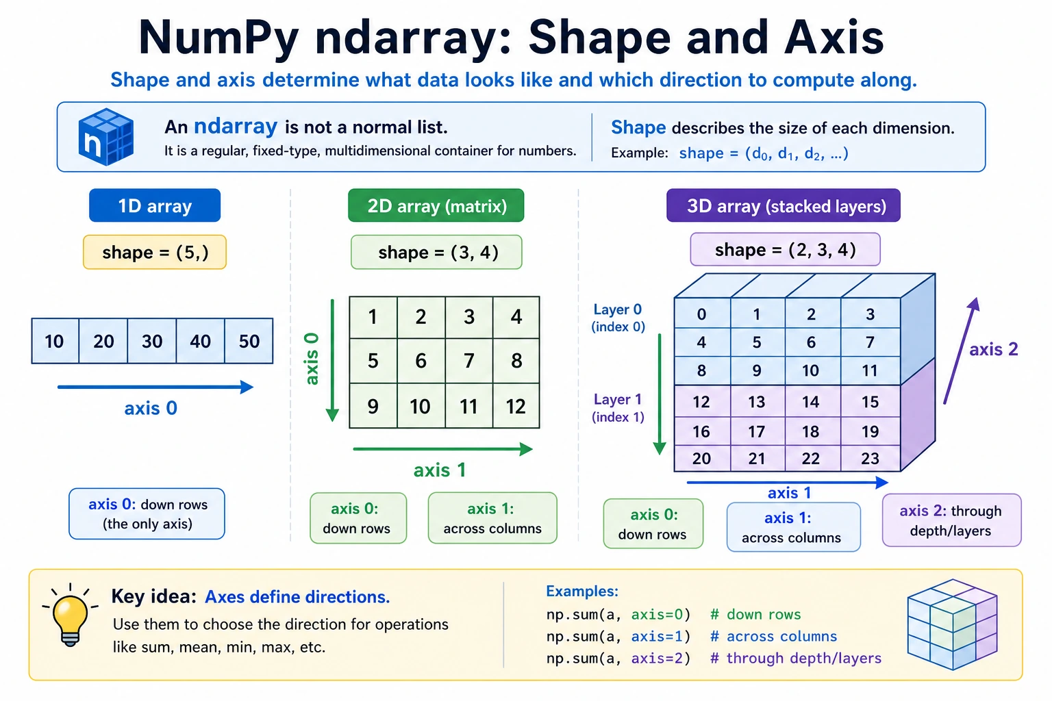
What shape Means

shape is one of the most commonly used attributes. It tells you the array's "shape":

# 1D array
a = np.array([1, 2, 3])
print(a.shape)      # (3,) → 3 elements

# 2D array
b = np.array([[1, 2, 3], [4, 5, 6]])
print(b.shape)      # (2, 3) → 2 rows and 3 columns

# 3D array
c = np.ones((2, 3, 4))
print(c.shape)      # (2, 3, 4) → 2 "matrices with 3 rows and 4 columns"

A good way to understand shape is: count layer by layer from outside to inside.

3D array shape = (2, 3, 4)
          ↓  ↓  ↓
          │  │  └── Innermost layer: 4 elements per row
          │  └───── Middle layer: 3 rows in each matrix
          └──────── Outermost layer: 2 matrices in total

---

Data Types (dtype)

All elements in a NumPy array must be of the same type. This is one of the reasons NumPy can run operations so quickly.

Common Data Types

dtype	Meaning	Example Values	Common Use
int32	32-bit integer	-2147483648 ~ 2147483647	Counting, indexing
int64	64-bit integer (default)	Larger range	General integers
float32	32-bit floating point	About 7 significant digits	Deep learning (saves memory)
float64	64-bit floating point (default)	About 15 significant digits	Scientific computing (high precision)
bool	Boolean	True / False	Conditional filtering
str_	String	"hello"	Text labels (less common)

Specifying a Data Type

# Let NumPy infer the type automatically
a = np.array([1, 2, 3])         # int64 (all integers)
b = np.array([1.0, 2.0, 3.0])   # float64 (contains decimal points)
c = np.array([1, 2.5, 3])       # float64 (mixed types are promoted automatically)

# Specify the type manually
d = np.array([1, 2, 3], dtype=np.float32)
print(d)        # [1. 2. 3.]
print(d.dtype)  # float32

e = np.zeros(5, dtype=np.int32)
print(e)        # [0 0 0 0 0]
print(e.dtype)  # int32

Type Conversion: astype

# Convert integers to floating-point numbers
int_arr = np.array([1, 2, 3, 4])
float_arr = int_arr.astype(np.float64)
print(float_arr)        # [1. 2. 3. 4.]
print(float_arr.dtype)  # float64

# Convert floating-point numbers to integers (truncates directly, not rounding!)
float_arr2 = np.array([1.7, 2.3, 3.9])
int_arr2 = float_arr2.astype(np.int32)
print(int_arr2)  # [1 2 3]  ← Note: 3.9 becomes 3, not 4!

# Boolean conversion
bool_arr = np.array([0, 1, 0, 2, -1]).astype(bool)
print(bool_arr)  # [False  True False  True  True]  ← 0 is False, non-zero is True

The Truncation Trap When Converting Float to Int

astype(int) directly truncates the decimal part, not round it. If you need rounding, use np.round() first:

arr = np.array([1.5, 2.3, 3.7])
print(arr.astype(int))     # [1 2 3] ← truncation
print(np.round(arr).astype(int))  # [2 2 4] ← round first, then convert

float32 vs float64: When Should You Use Each?

# float64: default, high precision
a = np.array([1.0, 2.0, 3.0])  # Default float64, 8 bytes per element

# float32: memory-saving, commonly used in deep learning
b = np.array([1.0, 2.0, 3.0], dtype=np.float32)  # 4 bytes per element

# Memory comparison
rng = np.random.default_rng(seed=42)
big_f64 = rng.random(1_000_000)                          # float64
big_f32 = rng.random(1_000_000).astype(np.float32)       # float32
print(f"float64 memory usage: {big_f64.nbytes / 1024 / 1024:.1f} MB")  # 7.6 MB
print(f"float32 memory usage: {big_f32.nbytes / 1024 / 1024:.1f} MB")  # 3.8 MB

Practical Advice

• In the data analysis stage: use the default float64, which has high precision and needs no extra effort
• In the deep learning stage: model parameters and data are usually float32 (or even float16), because GPU memory is precious
• For now, you only need to know that these two types exist; we will discuss them in more depth later in the deep learning section

---

Creating Arrays from Existing Arrays

Sometimes you need to create new arrays based on the shape of an existing array:

original = np.array([[1, 2, 3], [4, 5, 6]])

# Create an all-0 array with the same shape as original
z = np.zeros_like(original)
print(z)
# [[0 0 0]
#  [0 0 0]]

# Create an all-1 array with the same shape as original
o = np.ones_like(original)
print(o)
# [[1 1 1]
#  [1 1 1]]

# Create an array filled with a specified value with the same shape as original
f = np.full_like(original, 99)
print(f)
# [[99 99 99]
#  [99 99 99]]

# Create an uninitialized array (fast, but values are random)
e = np.empty_like(original)
# ⚠️ The values are random; do not use an empty array before assigning values!

---

Summary

---

Hands-On Practice

Exercise 1: Create Different Arrays

import numpy as np

# 1. Create a 1D array containing 1 to 20
arr1 = np.arange(1, 21)

# 2. Create a 4×5 all-zero matrix
arr2 = np.zeros((4, 5))

# 3. Create a 3×3 matrix where all elements are 7
arr3 = np.full((3, 3), 7)

# 4. Create 100 evenly spaced points between 0 and 2π (np.pi * 2)
arr4 = np.linspace(0, np.pi * 2, 100)

# 5. Create a 5×5 random integer matrix (range 1~50)
rng = np.random.default_rng(seed=42)
arr5 = rng.integers(1, 51, size=(5, 5))

Exercise 2: Check Attributes

Create an all-1 array with shape (3, 4, 5) and answer the following questions:

1. What is its dimension count (ndim)?
2. How many elements does it have (size)?
3. What is the default dtype?
4. After converting it to int32, how many bytes does each element take?

Exercise 3: Type Conversion

# Given exam scores (floating-point numbers)
scores = np.array([85.6, 92.3, 78.8, 95.1, 60.5, 73.9])

# 1. Round the scores to integers
rounded = np.rint(scores).astype(int)

# 2. Determine whether each score is passing (>= 60) to get a boolean array
passed = scores >= 60

# 3. Calculate the number of passing scores (hint: True counts as 1, False counts as 0)
pass_count = passed.sum()