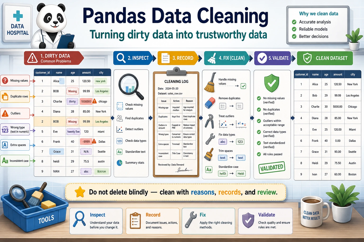
3.3.5 Data Cleaning

Section Positioning

When many beginners first learn data cleaning, the easiest misunderstanding is:

• Which function can get rid of dirty data

But a more solid understanding should be:

First identify the type of problem, then decide whether to delete, fill, modify, or keep it.

So the most important thing in this section is not memorizing functions, but building a cleaning sequence and a habit of judgment.

Learning Objectives

• Master strategies for detecting, deleting, and filling missing values
• Learn how to handle duplicate values
• Understand methods for outlier detection
• Master data type conversion and string processing

---

First, Build a Map

Data cleaning is better understood as “check first, then decide how to handle it”:

So what this section really wants to solve is:

• What are the most common problems in real data?
• When you first get dirty data, what is the safest order for checking it?

Why Do We Need Data Cleaning?

Real-world data is very dirty — missing values, duplicate rows, inconsistent formats, outliers... If you analyze it directly without cleaning, the results will definitely be unreliable.

"Data scientists spend 80% of their time cleaning data and 20% of their time complaining about cleaning data." — an industry saying

A Better Analogy for Beginners

You can think of data cleaning as:

• Washing, sorting, and preparing ingredients before cooking

You are not doing these steps just to make things “look neater”; you are doing them so that:

• when the real analysis starts later, you won’t be misled by broken, duplicated, or inconsistently formatted data

---

Handling Missing Values

Create Data with Missing Values

import pandas as pd
import numpy as np

df = pd.DataFrame({
    "Name": ["Alice", "Bob", "Carol", "David", "Eve"],
    "Age": [22, np.nan, 25, 28, np.nan],
    "City": ["Beijing", "Shanghai", None, "Shenzhen", "Hangzhou"],
    "Salary": [15000, 22000, np.nan, 35000, 12000]
})
print(df)

Detect Missing Values

# Check whether each position is missing
print(df.isna())        # True = missing (isnull() works the same)
print(df.notna())       # True = not missing

# Number of missing values in each column
print(df.isna().sum())
# Name      0
# Age       2
# City      1
# Salary    1

# Missing value ratio
print(df.isna().mean())
# Age       0.4
# City      0.2
# Salary    0.2

# Rows with missing values
print(df[df.isna().any(axis=1)])

Delete Missing Values

# Delete any row that contains missing values
df_cleaned = df.dropna()
print(df_cleaned)  # Only 2 rows remain (Alice, David)

# Delete rows where all values are missing
df.dropna(how="all")

# Look at specific columns only
df.dropna(subset=["Age"])         # Delete rows where Age is missing
df.dropna(subset=["Age", "Salary"]) # Delete rows where Age or Salary is missing

# Keep rows with at least N non-missing values
df.dropna(thresh=3)  # Keep only rows with at least 3 filled columns

Fill Missing Values

# Fill with a fixed value
df["City"].fillna("Unknown")

# Fill with mean (commonly used for numeric columns)
df["Age"].fillna(df["Age"].mean())

# Fill with median
df["Salary"].fillna(df["Salary"].median())

# Fill with the previous value (commonly used for time series)
df["Age"].ffill()    # forward fill

# Fill with the next value
df["Age"].bfill()    # backward fill

# Use different strategies for different columns
df_filled = df.fillna({
    "Age": df["Age"].median(),
    "City": "Unknown",
    "Salary": 0
})
print(df_filled)

Missing Value Handling Strategies

Strategy	Use Case	Method
Delete rows	Missing ratio is small (below 5%), data volume is large	dropna()
Fill with mean/median	Numeric data, symmetric distribution	fillna(mean/median)
Fill with mode	Categorical variables	fillna(mode()[0])
Forward/backward fill	Time series data	ffill() / bfill()
Fill with fixed value	Business rule is clear	fillna(0) or fillna("Unknown")
Interpolation	Continuous data	interpolate()

The Safest Default Order When Handling Missing Values for the First Time

A more reliable order is usually:

1. First check the missing-value ratio
2. Then decide whether the column is important
3. If only a little is missing, consider deleting rows
4. If a lot is missing, consider filling it

This is less likely to damage your data than calling dropna() immediately.

---

Handling Duplicate Values

df = pd.DataFrame({
    "Name": ["Alice", "Bob", "Alice", "Carol", "Bob"],
    "Department": ["Tech", "Marketing", "Tech", "Tech", "Marketing"],
    "Salary": [15000, 18000, 15000, 22000, 18000]
})

# Detect duplicate rows
print(df.duplicated())
# 0    False
# 1    False
# 2     True   ← Exactly the same as row 0
# 3    False
# 4     True   ← Exactly the same as row 1

# Number of duplicate rows
print(f"Number of duplicate rows: {df.duplicated().sum()}")  # 2

# Remove duplicate rows
df_unique = df.drop_duplicates()
print(df_unique)  # 3 rows

# Detect duplicates based on specific columns
df.drop_duplicates(subset=["Name"])        # Keep the first record for each name
df.drop_duplicates(subset=["Name"], keep="last")  # Keep the last record

What Are Duplicate Values Most Easily Misunderstood As?

Many beginners think “duplicate values = always delete them.” But a more careful way to think about it is:

• First confirm whether they are truly duplicates
• Or whether they are reasonable repeated records in the business context

For example:

• The same user placing multiple orders is not dirty data
• The same order being imported twice is the kind of duplicate that really needs cleaning

---

Handling Outliers

Z-score Method

rng = np.random.default_rng(seed=42)
df = pd.DataFrame({
    "Salary": np.concatenate([
        rng.normal(20000, 5000, 97),  # normal data
        np.array([100000, 150000, 200000])    # outliers
    ])
})

# Calculate Z-score
z_scores = (df["Salary"] - df["Salary"].mean()) / df["Salary"].std()

# |Z| > 3 is treated as an outlier
outliers = df[z_scores.abs() > 3]
print(f"Detected {len(outliers)} outliers")
print(outliers)

# Remove outliers
df_clean = df[z_scores.abs() <= 3]

IQR Method (More Robust)

Q1 = df["Salary"].quantile(0.25)
Q3 = df["Salary"].quantile(0.75)
IQR = Q3 - Q1

lower = Q1 - 1.5 * IQR
upper = Q3 + 1.5 * IQR

print(f"Normal range: [{lower:.0f}, {upper:.0f}]")

# Remove data outside the range
df_clean = df[(df["Salary"] >= lower) & (df["Salary"] <= upper)]

# Or clip outliers to the boundary
df["Salary_clipped"] = df["Salary"].clip(lower, upper)

A Simple Judgment Table for Beginners

Phenomenon	Safer First Reaction
Many missing values	First check whether the column can still be kept
Extremely unreasonable numeric values	First check whether it is a data entry error
The same row appears multiple times	First confirm whether it was imported twice
A column should be numeric but is a string	First perform type conversion

This table is especially useful for beginners because it breaks “dirty data” back down into several kinds of problems that can be handled separately.

---

Data Type Conversion

df = pd.DataFrame({
    "ID": ["001", "002", "003"],
    "Price": ["12.5", "23.8", "15.0"],
    "Quantity": ["3", "5", "2"],
    "Date": ["2024-01-15", "2024-02-20", "2024-03-10"]
})
print(df.dtypes)  # All object (strings)

# Convert data types
df["Price"] = df["Price"].astype(float)
df["Quantity"] = df["Quantity"].astype(int)
df["Date"] = pd.to_datetime(df["Date"])
print(df.dtypes)
# ID         object
# Price    float64
# Quantity    int64
# Date    datetime64[ns]

# Handle conversion errors
dirty = pd.Series(["10", "20", "abc", "40"])
# dirty.astype(int)  # ❌ Error

# Use to_numeric to handle it gracefully
clean = pd.to_numeric(dirty, errors="coerce")  # Values that cannot be converted become NaN
print(clean)
# 0    10.0
# 1    20.0
# 2     NaN
# 3    40.0

---

String Processing (str Accessor)

Pandas .str accessor lets you perform batch operations on an entire string column:

df = pd.DataFrame({
    "Name": ["  Alice ", "Bob", "  Carol  "],
    "Email": ["[email protected]", "[email protected]", "[email protected]"],
    "Phone": ["138-0000-1111", "139-2222-3333", "137-4444-5555"]
})

# Remove spaces
df["Name"] = df["Name"].str.strip()

# Convert to lowercase
df["Email"] = df["Email"].str.lower()

# Replace
df["Phone_clean"] = df["Phone"].str.replace("-", "")

# Contains check
print(df["Email"].str.contains("email"))  # All True

# Extract
df["Phone_prefix"] = df["Phone"].str[:3]

# Split
df["Email_username"] = df["Email"].str.split("@").str[0]

print(df)

Common str Methods

Method	Purpose	Example
.str.strip()	Remove leading and trailing spaces	" hello " → "hello"
.str.lower()	Convert to lowercase	"ABC" → "abc"
.str.upper()	Convert to uppercase	"abc" → "ABC"
.str.replace()	Replace text	"a-b".replace("-","")
.str.contains()	Check whether it contains a pattern	Returns a boolean Series
.str.startswith()	Check whether it starts with something	Returns a boolean Series
.str.len()	String length	"hello" → 5
.str.split()	Split	"a,b".split(",")
.str.extract()	Regex extraction	Extract the matched part

---

Practice: Clean a Dirty Dataset

import pandas as pd
import numpy as np

# Create a "dirty" dataset
dirty_data = pd.DataFrame({
    "Name": ["  Zhang San", "Li Si ", "Wang Wu", "Zhang San", " Zhao Liu", "Qian Qi", "Li Si"],
    "Age": [22, 28, np.nan, 22, "unknown", 150, 28],       # Missing, non-numeric, outlier
    "City": ["Beijing", "Shanghai ", None, "Beijing", " Guangzhou", "Shenzhen", "Shanghai"],
    "Salary": [15000, 22000, 18000, 15000, 20000, -5000, 22000]  # Negative value
})

print("=== Original Data ===")
print(dirty_data)
print(f"\nNumber of rows: {len(dirty_data)}")

# Step 1: Remove spaces from strings
dirty_data["Name"] = dirty_data["Name"].str.strip()
dirty_data["City"] = dirty_data["City"].str.strip()

# Step 2: Convert data types
dirty_data["Age"] = pd.to_numeric(dirty_data["Age"], errors="coerce")

# Step 3: Handle outliers
dirty_data.loc[dirty_data["Age"] > 120, "Age"] = np.nan    # Age > 120 is unreasonable
dirty_data.loc[dirty_data["Salary"] < 0, "Salary"] = np.nan      # Salary < 0 is unreasonable

# Step 4: Fill missing values
dirty_data["Age"] = dirty_data["Age"].fillna(dirty_data["Age"].median())
dirty_data["City"] = dirty_data["City"].fillna("Unknown")
dirty_data["Salary"] = dirty_data["Salary"].fillna(dirty_data["Salary"].median())

# Step 5: Remove duplicate rows
dirty_data = dirty_data.drop_duplicates()

print("\n=== After Cleaning ===")
print(dirty_data)
print(f"\nNumber of rows: {len(dirty_data)}")

What Is the Most Important Thing to Learn from This Mini Practice?

The most important thing is not the name of any single function, but the fact that cleaning usually follows a fairly reliable order:

1. Standardize the format first
2. Then convert types
3. Then handle outliers
4. Finally fill missing values and remove duplicates

Once the order is clear, many dirty-data problems become much easier to untangle.

A Data Cleaning Checklist Beginners Can Copy Directly

When you clean data for the first time, the safest checklist is usually:

1. Are the data types in each column correct?
2. Is the missing-value ratio high?
3. Are there obvious outliers?
4. Are there duplicate records?
5. Can the cleaning rules be explained to others?

The last point is especially important, because cleaning is also a kind of decision-making. If you can’t clearly explain why you deleted something or filled something in a certain way, it will be hard to make your analysis convincing.

---

Summary

Type	Detection	Handling Method
Missing values	isna(), info()	dropna(), fillna()
Duplicate values	duplicated()	drop_duplicates()
Outliers	Z-score, IQR	clip(), delete, replace with NaN
Type errors	dtypes	astype(), pd.to_numeric()
Dirty string data	Visual inspection, str.contains()	str.strip(), str.replace()

---

Hands-on Exercises

Exercise 1: Missing Value Handling

# Create a DataFrame with missing values (at least 20 rows and 5 columns)
# 1. Calculate the missing-value ratio for each column
# 2. Fill numeric columns with the median
# 3. Fill categorical columns with the mode
# 4. Delete columns with more than 50% missing values (if any)

Exercise 2: Complete Cleaning Workflow

# Create a dataset with various problems, then complete the full cleaning workflow:
# string spaces → type conversion → outlier handling → missing value filling → deduplication