3.3.4 Data Selection and Filtering

Where this section fits

When many beginners first learn Pandas, what usually blocks them is not cleaning, but:

• How do I select the part of the data I actually want?

So the most important thing in this section is not memorizing every syntax pattern, but building this first question:

Am I selecting by label, by position, or by condition?

Learning Objectives

• Master loc (label indexing) and iloc (position indexing)
• Learn to use boolean indexing for conditional filtering
• Master the query() method
• Learn multi-condition filtering

---

First, build a mental map

Data selection and filtering are easier to understand as “who do I want to select?”

So what this section really aims to solve is:

• In different scenarios, should you think of loc, iloc, or boolean indexing first?
• Why is the first step in so many Pandas problems to “select the data you need first”?

Prepare sample data

import pandas as pd
import numpy as np

df = pd.DataFrame({
    "Name": ["Alice", "Bob", "Charlie", "Diana", "Ethan", "Fiona"],
    "Age": [22, 28, 25, 35, 21, 30],
    "Department": ["Engineering", "Marketing", "Engineering", "Management", "Engineering", "Marketing"],
    "Salary": [15000, 18000, 22000, 35000, 12000, 20000],
    "HireYear": [2023, 2020, 2021, 2018, 2024, 2019]
})
print(df)

A better analogy for beginners

You can think of this section as:

• Finding the rows and columns you really want in a large table

In other words, the core of this section is not “many syntax patterns,” but:

• First figure out whether you are searching by name
• Or by position
• Or filtering by condition

---

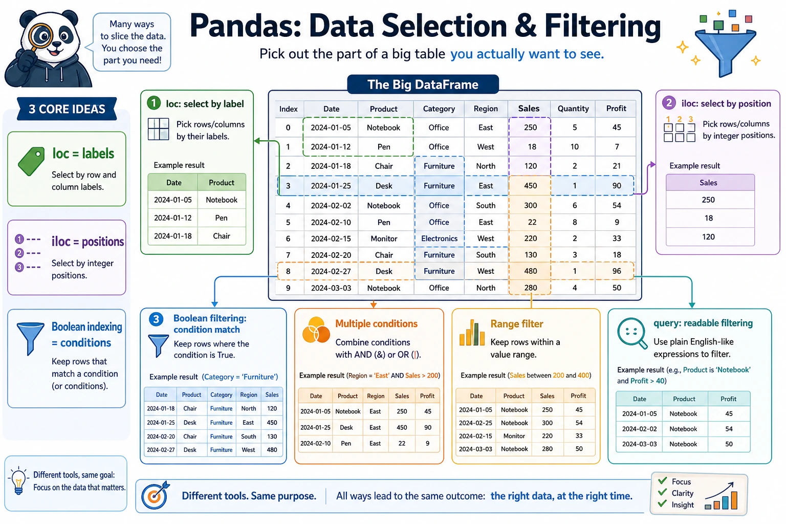
loc: label indexing

loc uses labels (names) to locate data, with the format: df.loc[row_label, column_label]

What should you remember first when learning loc?

The most important thing to remember first is:

loc selects by “name and label.”

That means it is more like:

• I know which column I want, and which label range I want

# Select a single row
print(df.loc[0])         # The first row (the row with label 0)

# Select multiple rows
print(df.loc[0:2])       # Labels 0 to 2 (includes 2!)

# Select specific rows and columns
print(df.loc[0, "Name"])          # "Alice"
print(df.loc[0:2, "Name"])        # Names in the first 3 rows
print(df.loc[0:2, ["Name", "Salary"]])  # Names and salaries in the first 3 rows

# Select certain columns from all rows
print(df.loc[:, ["Name", "Age"]])

# Conditional filtering (the most common use!)
print(df.loc[df["Age"] > 25])    # All rows where age is greater than 25

---

iloc: position indexing

iloc uses position (integer) to locate data, following the same slicing rules as Python lists:

What should you remember first when learning iloc?

The most important thing to remember first is:

iloc selects by “which row, which column.”

So it is more like:

• You use coordinates to pick values from the table

# Select a single row
print(df.iloc[0])        # First row

# Select multiple rows (does not include the end, just like Python)
print(df.iloc[0:3])      # Rows 0, 1, 2

# Select specific positions
print(df.iloc[0, 0])     # Row 0, column 0 → "Alice"
print(df.iloc[0:3, 0:2]) # First 3 rows, first 2 columns
print(df.iloc[[0, 2, 4]])  # Rows 0, 2, 4

# Select the last row
print(df.iloc[-1])

loc vs iloc comparison

Feature	loc	iloc
Indexing method	Label (name)	Position (integer)
Slice end	Included	Not included
Example	df.loc[0:2] → 3 rows	df.iloc[0:2] → 2 rows
Conditional filtering	✅ Supported	❌ Not supported

Most common pitfall

When the index is the default 0, 1, 2..., loc[0:2] returns 3 rows, while iloc[0:2] returns 2 rows.

print(len(df.loc[0:2]))    # 3  (includes label 2)
print(len(df.iloc[0:2]))   # 2  (does not include position 2)

A selection table that beginners can remember first

What you are thinking	Safer first choice
I know the column name or label	loc
I only know which row and column position	iloc
I want to filter people or orders by a condition	Boolean indexing
The condition is long and I want it to read more like a sentence	query()

This table is especially good for beginners because it turns “which one should I use?” into a question you can actually answer.

---

Boolean indexing: conditional filtering

This is the most frequently used operation in data analysis:

Why is boolean indexing so important?

Because in real analysis tasks, what you most often do is:

• Find orders with amount greater than a certain value
• Find people in a specific department
• Find a subset that meets two or three conditions

In other words, in many analysis tasks, the first real step is:

• First filter out the data you want to analyze

Single-condition filtering

# Employees with salary greater than 20000
high_salary = df[df["Salary"] > 20000]
print(high_salary)

# Employees in the "Engineering" department
tech = df[df["Department"] == "Engineering"]
print(tech)

# Employees whose age is not 22
print(df[df["Age"] != 22])

Combining multiple conditions

# Engineering department and salary greater than 15000 (use & for AND)
result = df[(df["Department"] == "Engineering") & (df["Salary"] > 15000)]
print(result)

# Engineering department or management department (use | for OR)
result = df[(df["Department"] == "Engineering") | (df["Department"] == "Management")]
print(result)

# Negation (use ~ for NOT)
result = df[~(df["Department"] == "Engineering")]  # Non-engineering departments
print(result)

Multiple conditions must use parentheses

Just like with NumPy, every condition must be wrapped in parentheses. Use &, |, and ~ instead of and, or, and not.

# ❌ Wrong
df[df["Age"] > 25 and df["Salary"] > 20000]

# ✅ Correct
df[(df["Age"] > 25) & (df["Salary"] > 20000)]

isin: match multiple values

# Employees whose department is in ["Engineering", "Marketing"]
result = df[df["Department"].isin(["Engineering", "Marketing"])]
print(result)

# Reverse: not in these departments
result = df[~df["Department"].isin(["Engineering", "Marketing"])]
print(result)

between: range filtering

# Ages between 22 and 30 (inclusive)
result = df[df["Age"].between(22, 30)]
print(result)

String conditions

# Names containing "li"
result = df[df["Name"].str.contains("li")]

# Names starting with "A"
result = df[df["Name"].str.startswith("A")]

The safest default order when you first do filtering problems

A safer order is usually:

1. Ask yourself whether you are selecting by label, by position, or by condition
2. Use boolean indexing first when the condition is simple
3. Consider query() when the condition is long
4. Finally, combine row selection and column selection

This is usually less confusing than mixing several styles at once from the start.

---

The query() method

query() lets you filter data in a way that feels closer to natural language:

# Equivalent to df[df["Salary"] > 20000]
result = df.query("Salary > 20000")
print(result)

# Multiple conditions
result = df.query("Department == 'Engineering' and Salary > 15000")
print(result)

# Using variables
min_salary = 20000
result = df.query("Salary > @min_salary")  # @ references an external variable
print(result)

# Range query
result = df.query("22 <= Age <= 30")
print(result)

When should you use query()?

• For simple conditions: boolean indexing like df[df["col"] > 5] is more direct
• For complex conditions: query() is more readable, especially with multiple conditions
• When you need to reference variables: query("col > @var") is very convenient

---

Summary of methods for selecting specific data

A data selection checklist beginners can copy directly

When you first do a Pandas filtering problem, the safest checklist is usually:

1. Am I selecting columns, rows, or both rows and columns?
2. Am I selecting by label, by position, or by condition?
3. Did I add parentheses to the conditions?
4. Is the result really the rows and columns I expected?

If you answer these 4 questions clearly, many filtering problems become much easier.

---

Practice: data filtering

import pandas as pd
import numpy as np

# Create a set of e-commerce order data
rng = np.random.default_rng(seed=42)
n = 100
orders = pd.DataFrame({
    "OrderID": range(1001, 1001 + n),
    "Customer": rng.choice(["Alice", "Bob", "Charlie", "Diana", "Eve"], n),
    "Category": rng.choice(["Electronics", "Clothing", "Food", "Books"], n),
    "Amount": rng.integers(10, 500, n),
    "Quantity": rng.integers(1, 10, n),
    "Returned": rng.choice([True, False], n, p=[0.1, 0.9])
})

# View the data
print(orders.head(10))
print(orders.info())

# Filtering practice
# 1. Orders with amount greater than 300
print(orders[orders["Amount"] > 300])

# 2. Electronic products purchased by Alice
print(orders.query("Customer == 'Alice' and Category == 'Electronics'"))

# 3. Orders that have not been returned and are in the top 10 by amount
not_returned = orders[~orders["Returned"]]
top10 = not_returned.nlargest(10, "Amount")
print(top10[["OrderID", "Customer", "Amount"]])

---

Hands-on exercises

Exercise 1: Basic filtering

# Use the orders data above
# 1. Find all returned orders
# 2. Find the number of orders with amounts between 100 and 200
# 3. Find orders in the "Books" or "Food" category
# 4. Find the average amount of Bob's non-returned orders

Exercise 2: Comprehensive filtering

# 1. What is the maximum order amount for each customer? (Hint: filter first, then aggregate)
# 2. Which customers have return records?
# 3. Which orders are in the top 5% by amount? (Hint: use quantile)

What you should take away from this section

• loc selects by label, iloc selects by position, and boolean indexing selects by condition
• In many real analysis tasks, the first step is not calculation, but filtering
• Before writing code, clearly think about “who do I want to select?” — that is more reliable than memorizing syntax