5.1.5 Main Thread of Major Breakthroughs in Machine Learning History
This section is not about memorizing years. Instead, it helps you understand:
- What people were stuck on before each machine learning breakthrough
- What problem the new method actually solved
- Where it fits in this chapter
- What engineering capability this historical milestone becomes in real projects
First, grasp the main thread of machine learning history in one sentence
You can first understand the history of machine learning as a path from “handwritten rules” to “learning patterns from data.”
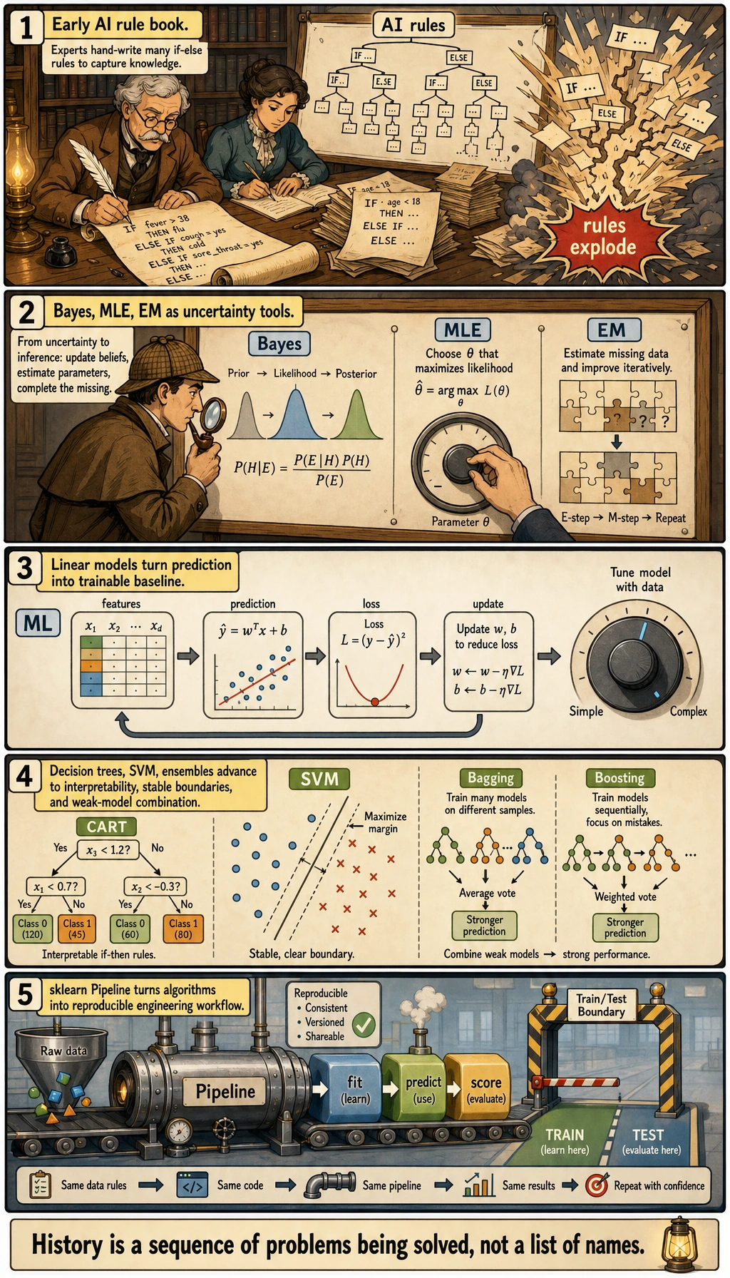
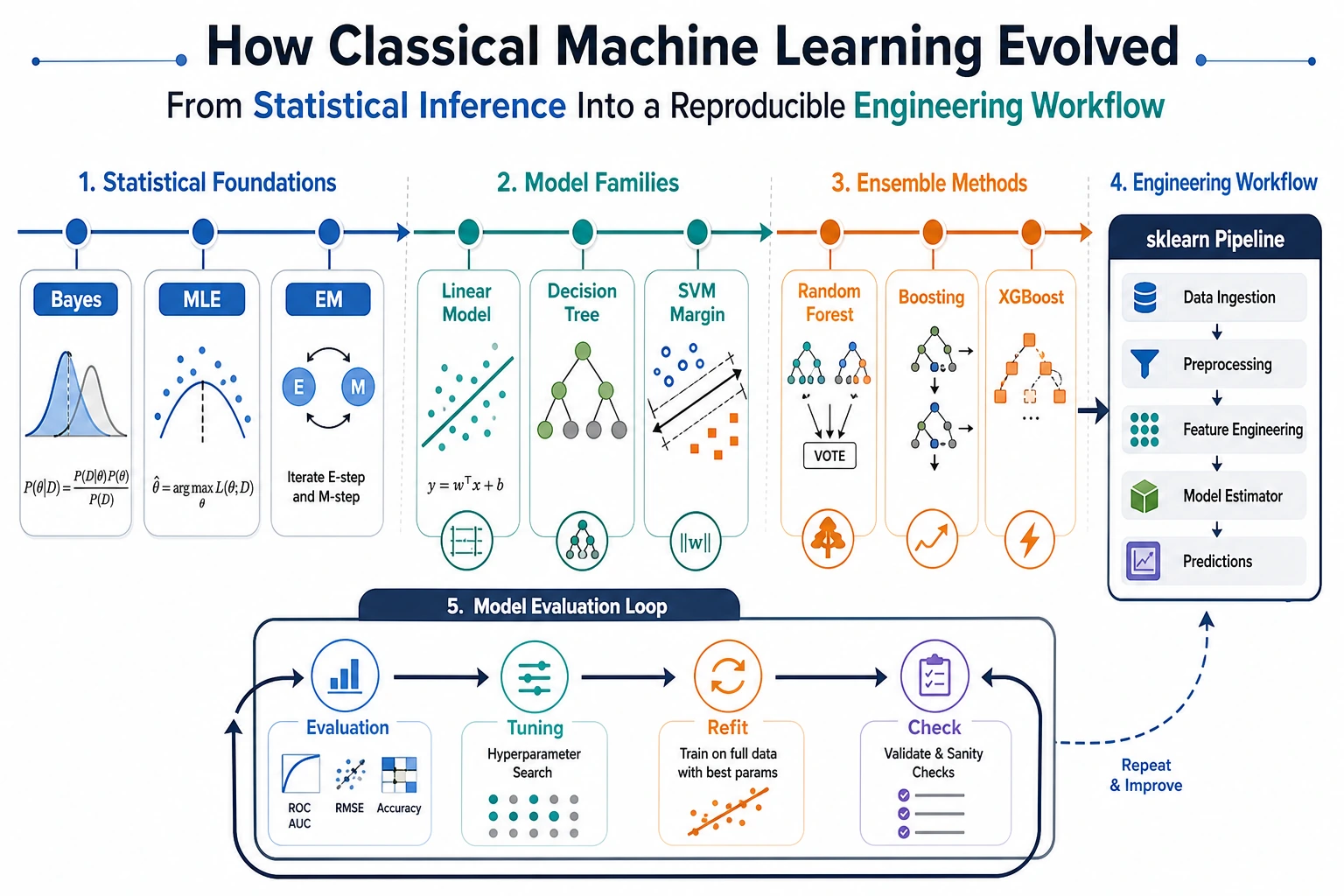
Read the comic as a problem chain: handwritten rules became too brittle, probability made uncertainty usable, linear models made training concrete, trees/SVM/ensembles improved structure and stability, and sklearn turned these ideas into a repeatable workflow.
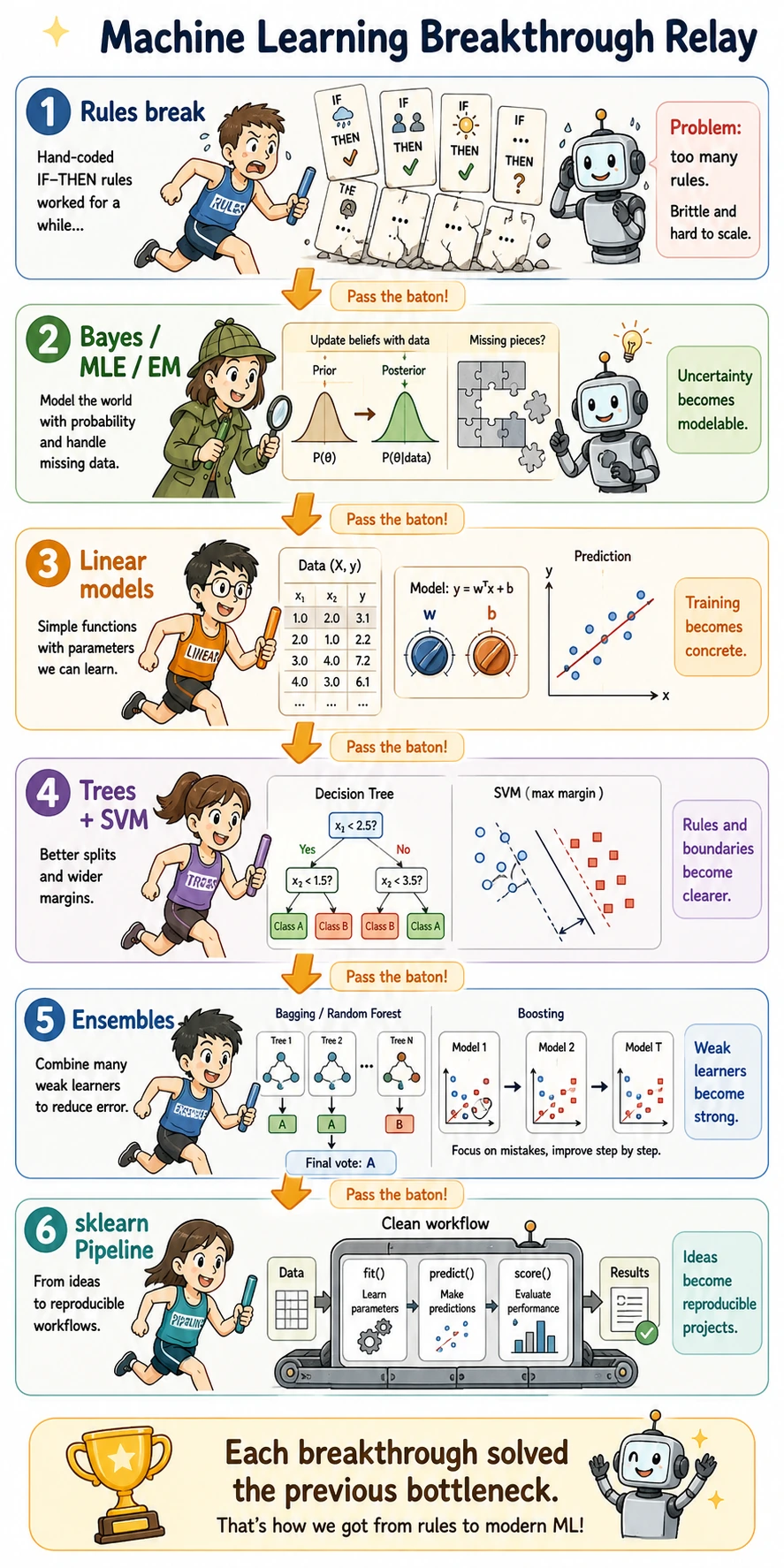
This relay view is useful because every breakthrough hands the baton to the next one. Probability methods made uncertainty usable; linear models made training visible; trees and SVMs made structure and boundaries clearer; ensembles made unstable models stronger; sklearn finally made the whole process reproducible.
Early AI relied heavily on manual rules. Human experts wrote knowledge as if-else logic or symbolic rules, and the system reasoned according to those rules. This approach works in scenarios with clear rules, but once the task becomes complex, the rules explode in number. For example, if you want to determine whether an email is spam, it is very hard to write out all the rules in advance.
The key shift in machine learning is: instead of writing rules directly, prepare data, define the objective, choose a model, and let the model learn patterns from examples by itself. What Chapter 5 trains is not “memorizing algorithm names,” but this modeling mindset:
| Historical change | Capability in this chapter |
|---|---|
| From rules to data | Know when machine learning should be used |
| From one-time fitting to evaluation | Learn train/test, metrics, and generalization |
| From a single model to model families | Compare baseline, tree models, and ensemble methods |
| From handwritten workflows to engineering | Use sklearn, Pipeline, and reports to review projects |
Keyword decoder for this history page
| Keyword | Full name / meaning | Beginner-friendly explanation |
|---|---|---|
AI | Artificial Intelligence | The broader goal: make machines show intelligent behavior |
ML | Machine Learning | A branch of AI where models learn patterns from data instead of only following handwritten rules |
MLE | Maximum Likelihood Estimation | Choose the parameters that make the observed data look most likely |
EM | Expectation-Maximization | Alternate between guessing hidden information and updating parameters |
SVM | Support Vector Machine | A classifier that prefers a wide, stable margin between classes |
CART | Classification and Regression Trees | A systematic way to build decision trees for classification and regression |
Bagging | Bootstrap Aggregating | Train many models in parallel on sampled data, then vote or average |
Boosting | Sequential error correction | Train models one after another, each focusing more on previous mistakes |
GBDT | Gradient Boosting Decision Tree | A Boosting family that improves predictions with many small trees |
XGBoost | Extreme Gradient Boosting | A fast, production-friendly implementation of GBDT-style ideas |
baseline | First reasonable comparison model | A simple model you beat before claiming progress |
Pipeline | Reproducible chain of steps | Keeps preprocessing, training, and prediction connected in the same order |
Breakthrough 1: Bayes, maximum likelihood, and EM made “uncertainty” modelable
In many real-world problems, data is not absolutely certain. Users hesitate, sensors contain noise, samples may be missing, and labels may be imperfect.
At this point, machine learning needs to answer one question:
How do we make the most reasonable judgment when information is incomplete and noisy?
Bayes’ rule provides a way to update judgments after seeing new evidence. Maximum likelihood estimation lets us infer the most likely parameters based on observed data. The EM algorithm handles a more difficult situation: when there are hidden variables or missing information in the data, it first estimates the hidden part, then updates the parameters, and repeats this process iteratively.
For beginners, you can think of them like this:
| Method | Everyday analogy | Connection in this chapter |
|---|---|---|
| Bayes | A detective updates the probability of a suspect after seeing new evidence | Probability intuition, optional Naive Bayes |
| MLE | Infer the most likely demand pattern from past sales | Loss functions, parameter estimation |
| EM | Assemble a puzzle with a few missing pieces: guess the missing parts first, then refine the whole picture | Clustering, background of latent variable models |
This group of methods may not all be deeply derived in the main line of Chapter 5, but they explain why machine learning cannot do without probability, loss, and parameter estimation.
Suggested study mapping:
| Corresponding section | What you should take away |
|---|---|
| Chapter 4 Probability and Statistics | Probability is not just an exam topic; it is the language for expressing uncertainty |
| Section 1.5 How mathematics truly flows into machine learning | How parameters, loss, and optimization connect to the training loop |
| Optional module: classical ML | How traditional methods such as Naive Bayes and LDA use probabilistic thinking |
Breakthrough 2: Linear models turned “prediction” into a trainable baseline
Linear regression and logistic regression look simple, but they are extremely important in machine learning because they let beginners see a complete training structure for the first time:
- Input features
- Compute predictions
- Measure error
- Adjust parameters
- Evaluate on the test set
Linear regression solves continuous-value prediction, while logistic regression solves classification probabilities. They are not “outdated algorithms”; they are the backbone of many complex models. Neural networks can also be understood as stacks of many linear transformations plus nonlinear activations.
Suggested study mapping:
| Corresponding section | Learning focus brought by this historical breakthrough |
|---|---|
| 2.2 Linear Regression | Understand for the first time “model, loss, parameter updates” |
| 2.3 Logistic Regression | Move from continuous prediction to classification probabilities and decision boundaries |
| Chapter 6 Neural Networks | Understand why neurons are like “trainable linear models + activation functions” |
Breakthrough 3: Decision trees made machine learning results look more like human-readable rules
Linear models are stable, but they are often not intuitive enough and are not good at expressing complex nonlinear rules. The breakthrough of decision trees is:
Organize learned patterns into a sequence of interpretable decisions.
You can think of a decision tree as a “20 Questions” game. Each time, the model chooses a feature to split on, making the samples in each node purer and purer. Methods such as CART systematized classification trees and regression trees, making tree models one of the most interpretable types of models in machine learning.
But a single tree also has an obvious problem: it can easily grow too deep and memorize noise in the training set. This naturally leads to random forests and Boosting.
Suggested study mapping:
| Corresponding section | Learning focus brought by this historical breakthrough |
|---|---|
| 2.4 Decision Trees | Rule splitting, purity, pruning, and interpretability |
| 4.3 Bias-variance | Why deep trees overfit |
| 5.5 Pipeline | How to place tree models into a complete modeling workflow |
Breakthrough 4: SVM clearly explained the idea that the decision boundary should be stable
The core story of SVM is very suitable for beginners to understand classification boundaries.
If two lines can separate the samples, which one is better? SVM’s answer is:
Choose the boundary that stays as far away as possible from both classes of samples.
This is the idea of maximum margin. It helps the model avoid making risky splits that hug the training samples too closely, and instead leave as much safety margin as possible. Kernel methods further allow SVM to handle nonlinear boundaries.
SVM may not be the first choice for every project today, but it is historically very important because it explains “generalization boundaries” and “stable classification” so elegantly.
Suggested study mapping:
| Corresponding section | Learning focus brought by this historical breakthrough |
|---|---|
| Optional module: SVM | Maximum margin, support vectors, kernel methods |
| Model evaluation in this chapter | A high training score does not necessarily mean a stable boundary |
| Feature engineering in this chapter | SVM is sensitive to feature scaling |
Breakthrough 5: Random forests and Boosting combined weak models into strong models
A single tree can easily overfit, but trees have one huge advantage: they can handle nonlinearity and feature interactions. So machine learning entered a very important stage:
Stop worshiping a single model; combine multiple models instead.
Random forests use the idea of Bagging to train many trees in parallel, then vote or average to reduce the instability of a single tree. Boosting trains models sequentially, focusing on the samples that previous models got wrong and correcting errors step by step.
This path has a huge impact on industrial machine learning, especially for tabular data tasks. Tools such as XGBoost, LightGBM, and CatBoost make Boosting a strong baseline in real projects and competitions.
Suggested study mapping:
| Corresponding section | Learning focus brought by this historical breakthrough |
|---|---|
| 2.5 Ensemble Learning | The difference between Bagging and Boosting |
| 4.1 Metric selection | Even strong models must be compared under the right metric |
| 6.4 Kaggle introduction | Why tabular data projects often start with XGBoost-like models |
Breakthrough 6: sklearn turned classical machine learning into a unified engineering workflow
Algorithmic breakthroughs are important, but engineering matters too. The value of scikit-learn is not only that it provides many models, but also that it unifies classical machine learning into a very stable interface:
model.fit(X_train, y_train)
pred = model.predict(X_test)
score = metric(y_test, pred)
This allows beginners to first learn a unified workflow, and then gradually understand the differences between models. It also makes projects easier to reproduce, compare, and organize.
Suggested study mapping:
| Corresponding section | Learning focus brought by this historical breakthrough |
|---|---|
| 1.4 Introduction to the Scikit-learn framework | The unified mental model of fit / predict / score |
| 5.5 Pipeline | Prevent data leakage and messy workflows |
| Stage 6 projects | Turn training, evaluation, and reporting into reproducible projects |
Assign the historical breakthroughs to the Chapter 5 learning path
You can return to the specific sections according to the table below:
| Historical breakthrough | Problem it solved | Corresponding course section |
|---|---|---|
| Bayes / MLE / EM | Uncertainty, parameter estimation, latent variables | Chapter 4 Probability and Statistics, Section 1.5, optional classical ML |
| Linear Regression | The simplest trainable model for continuous-value prediction | 2.2 Linear Regression |
| Logistic Regression | Classification probabilities and linear decision boundaries | 2.3 Logistic Regression |
| CART / Decision Trees | Interpretable rules and nonlinear splits | 2.4 Decision Trees |
| SVM | Maximum margin and stable classification boundaries | Optional module: classical ML |
| Random Forest | Voting across many trees to reduce variance | 2.5 Ensemble Learning |
| AdaBoost / GBDT / XGBoost | Sequential error correction to improve tabular baselines | 2.5 Ensemble Learning, 6.4 Kaggle |
| sklearn / Pipeline | Organize algorithms into a reproducible engineering workflow | 1.4 sklearn, 5.5 Pipeline |
The intuition you should form after finishing this section
The history of machine learning is not just a list of “old algorithms,” but a process in which problems were gradually solved:
| Old problem | New breakthrough | Capability you should practice now |
|---|---|---|
| Humans cannot finish writing all the rules | Learn patterns from data | Define tasks and prepare data |
| A single score is not trustworthy | train/test and cross-validation | Judge whether a model generalizes |
| A single model is unstable | Ensemble learning | Compare baseline and strong models |
| Workflows become messy easily | sklearn / Pipeline | Build reproducible modeling projects |
After finishing this section, when you study linear regression, decision trees, ensemble learning, and evaluation, it will be easier to understand: these technologies did not suddenly appear as isolated terms. They were all introduced to solve real problems that kept reappearing throughout the history of machine learning.