5.2.6 SVM: Maximum Margin and Kernel Methods

Section Position

SVM is not always the first production model today, but it is still one of the clearest ways to learn margin, kernel, and distance-sensitive modeling.

What You Will Build

This lesson turns SVM into a small lab. You will:

• compare linear and rbf kernels on a curved dataset;
• prove why StandardScaler matters for SVM;
• tune C and gamma and inspect support vector counts;
• learn when SVM is worth trying and when ensembles are usually easier.

The practical sentence to remember:

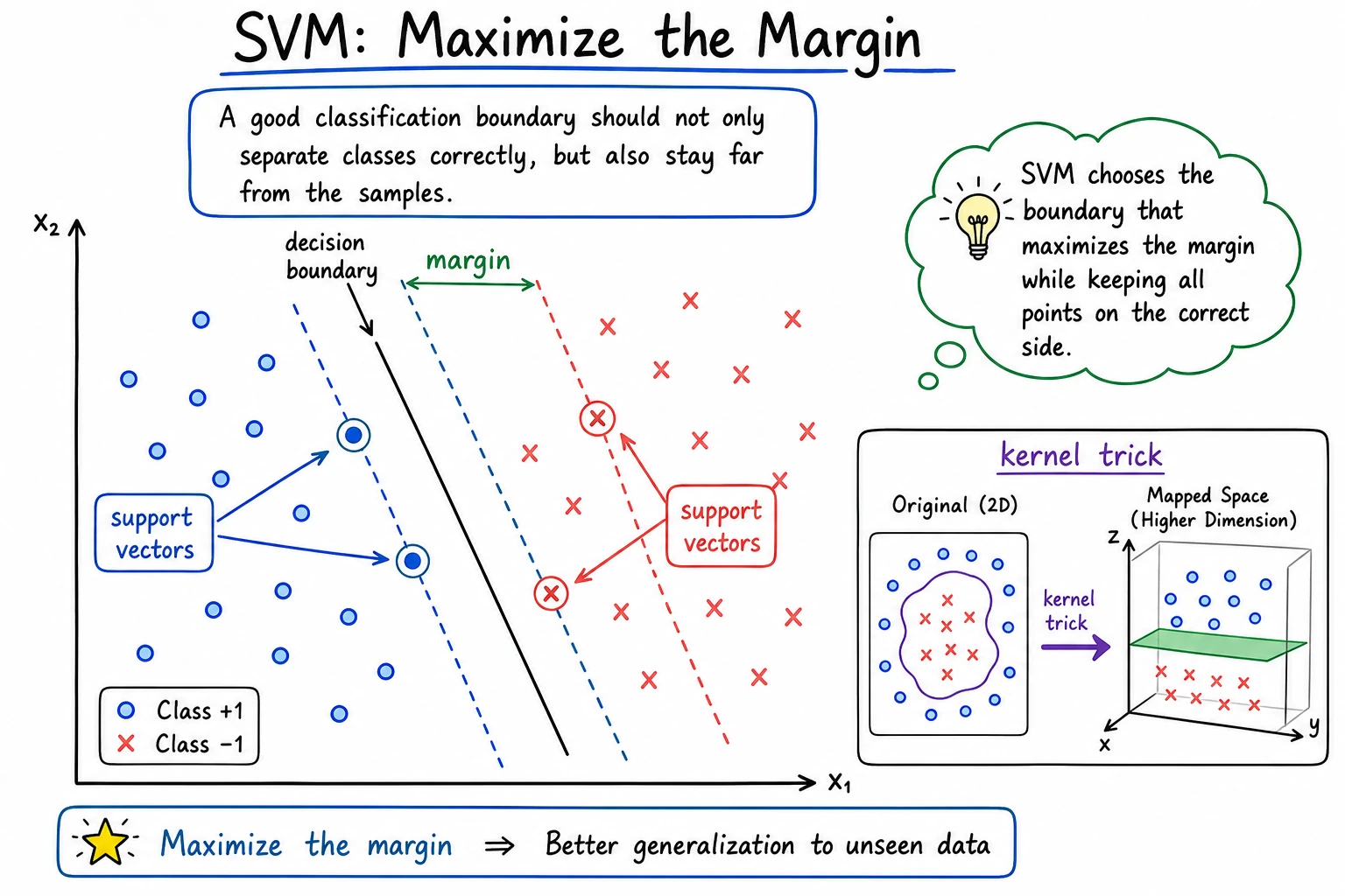
SVM does not only ask "did I classify this correctly?" It asks "can I place the boundary with enough room around the closest samples?"

Keyword Decoder

Term	Practical meaning
SVM	Support Vector Machine, a classifier that searches for a large-margin boundary
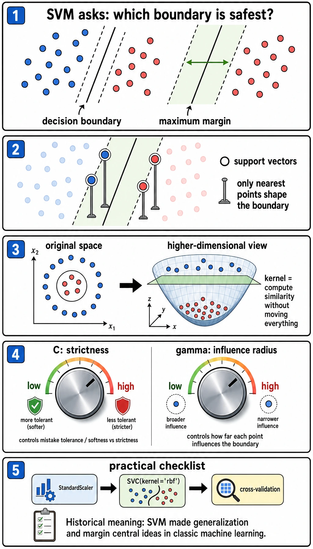
margin	Distance between the boundary and the closest samples
support vector	A training sample close enough to shape the boundary
kernel	A similarity function that lets SVM create nonlinear boundaries
RBF	Radial Basis Function, a common nonlinear kernel
C	Mistake penalty; larger C tries harder to fit training points
gamma	Local influence radius for the RBF kernel; larger values create more local boundaries
SVC	sklearn's Support Vector Classifier

Setup

python -m pip install -U scikit-learn

SVM is sensitive to feature scale, so the examples use Pipeline(StandardScaler(), SVC(...)). This is not decoration; it is part of the model workflow.

Run the Complete Lab

Create svm_lab.py:

from itertools import product
from sklearn.datasets import make_moons
from sklearn.metrics import accuracy_score
from sklearn.model_selection import train_test_split
from sklearn.pipeline import make_pipeline
from sklearn.preprocessing import StandardScaler
from sklearn.svm import SVC


X, y = make_moons(n_samples=400, noise=0.25, random_state=42)
X_train, X_test, y_train, y_test = train_test_split(
    X, y, test_size=0.25, random_state=42, stratify=y
)

print("kernel_comparison")
for kernel in ["linear", "rbf"]:
    model = make_pipeline(StandardScaler(), SVC(kernel=kernel, C=1.0, gamma="scale"))
    model.fit(X_train, y_train)
    svc = model.named_steps["svc"]
    print(
        f"kernel={kernel:<6} "
        f"accuracy={accuracy_score(y_test, model.predict(X_test)):.3f} "
        f"support_vectors={int(svc.n_support_.sum())}"
    )

print("scaling_check")
X_bad_scale = X.copy()
X_bad_scale[:, 1] *= 100
X_train2, X_test2, y_train2, y_test2 = train_test_split(
    X_bad_scale, y, test_size=0.25, random_state=42, stratify=y
)
raw = SVC(kernel="rbf", C=1.0, gamma="scale")
raw.fit(X_train2, y_train2)
scaled = make_pipeline(StandardScaler(), SVC(kernel="rbf", C=1.0, gamma="scale"))
scaled.fit(X_train2, y_train2)
print(f"without_scaling={accuracy_score(y_test2, raw.predict(X_test2)):.3f}")
print(f"with_scaling={accuracy_score(y_test2, scaled.predict(X_test2)):.3f}")

print("c_gamma_lab")
for C, gamma in product([0.1, 1.0, 10.0], [0.1, 1.0]):
    model = make_pipeline(StandardScaler(), SVC(kernel="rbf", C=C, gamma=gamma))
    model.fit(X_train, y_train)
    svc = model.named_steps["svc"]
    print(
        f"C={C:<4} gamma={gamma:<3} "
        f"accuracy={accuracy_score(y_test, model.predict(X_test)):.3f} "
        f"support_vectors={int(svc.n_support_.sum())}"
    )

Run it:

python svm_lab.py

Expected output:

kernel_comparison
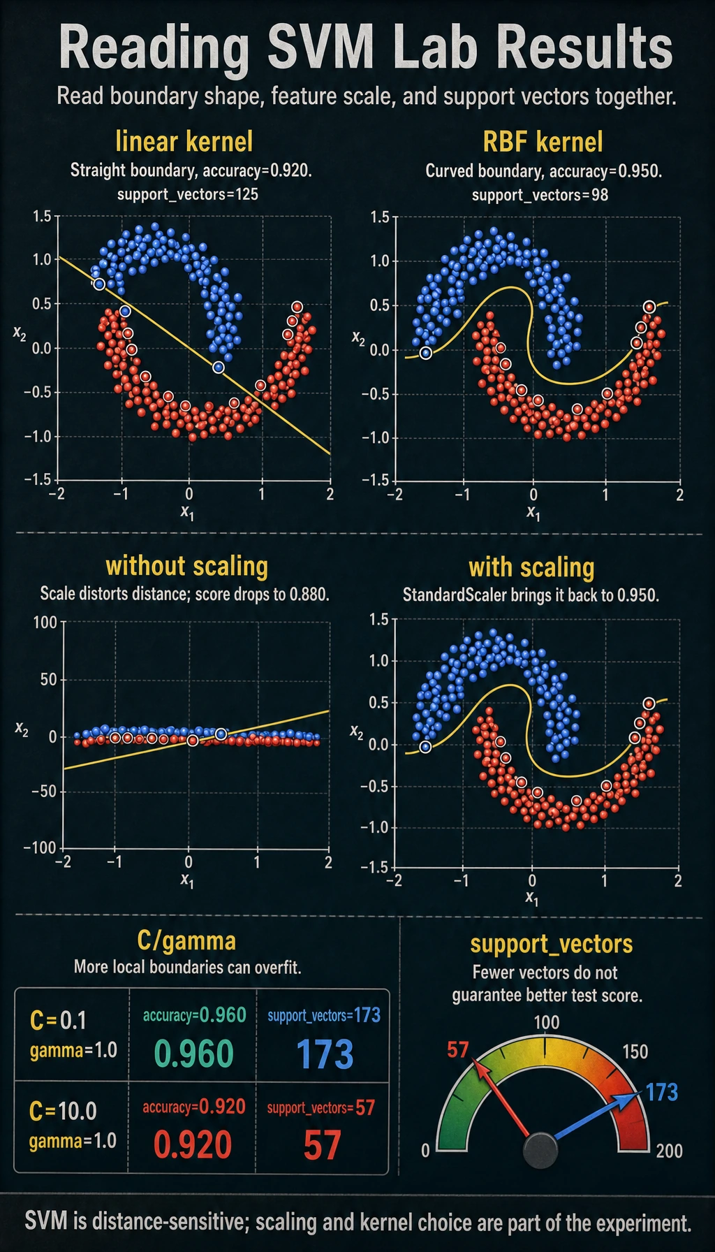
kernel=linear accuracy=0.920 support_vectors=125
kernel=rbf    accuracy=0.950 support_vectors=98
scaling_check
without_scaling=0.880
with_scaling=0.950
c_gamma_lab
C=0.1  gamma=0.1 accuracy=0.940 support_vectors=187
C=0.1  gamma=1.0 accuracy=0.960 support_vectors=173
C=1.0  gamma=0.1 accuracy=0.950 support_vectors=134
C=1.0  gamma=1.0 accuracy=0.930 support_vectors=87
C=10.0 gamma=0.1 accuracy=0.960 support_vectors=111
C=10.0 gamma=1.0 accuracy=0.920 support_vectors=57

Read the Kernel Result

The curved make_moons dataset is intentionally hard for a straight boundary:

kernel=linear accuracy=0.920 support_vectors=125
kernel=rbf    accuracy=0.950 support_vectors=98

The linear kernel asks for a straight separating line. The rbf kernel compares local similarity, so it can create a curved boundary. Use this simple rule:

Situation	First SVM choice
Boundary looks roughly straight	kernel="linear"
Boundary is curved and the dataset is not huge	kernel="rbf"
You have many rows or many features	Try logistic regression, linear SVM, or tree ensembles first

Why Scaling Is Not Optional

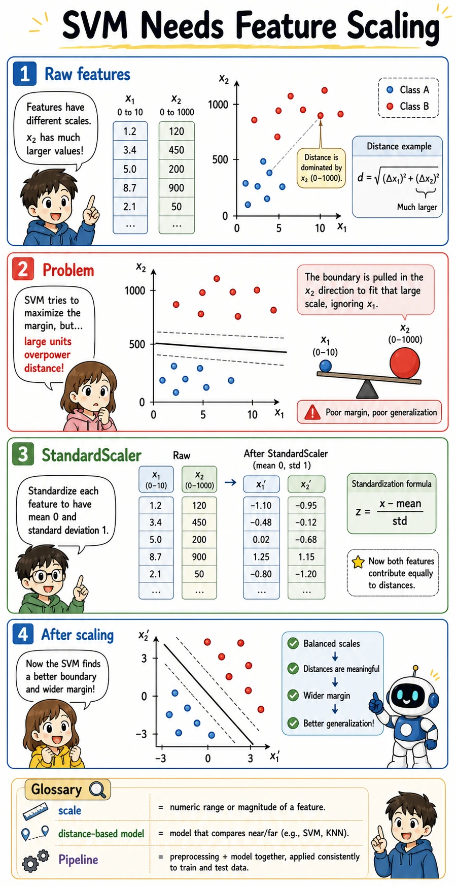
SVM relies on distances and similarities. If one feature has values around 0-1 and another has values around 0-1000, the larger-scale feature can dominate the boundary even when it is not more meaningful.

The lab makes that problem visible:

without_scaling=0.880
with_scaling=0.950

This is why StandardScaler should live inside a Pipeline: the scaler is fitted only on the training fold, then applied safely to validation/test data.

Understand C and gamma

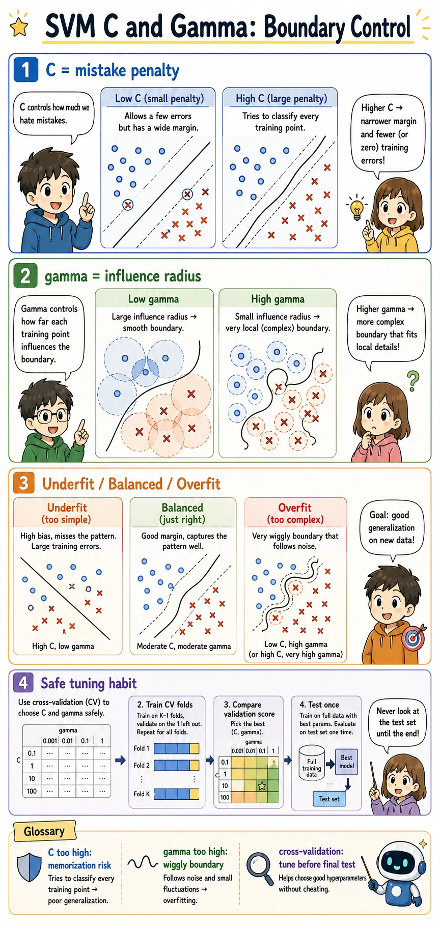
C and gamma control different parts of the boundary:

Parameter	If too small	If too large
C	allows more mistakes; wider, smoother margin	chases training points more aggressively
gamma	influence is broad; boundary may be too smooth	influence is local; boundary can become wiggly

Read the output with two signals:

C=0.1  gamma=1.0 accuracy=0.960 support_vectors=173
C=10.0 gamma=1.0 accuracy=0.920 support_vectors=57

The second model uses fewer support vectors, but its test accuracy is worse. Fewer support vectors is not automatically better. It can mean the model is using a sharper boundary that generalizes poorly.

For experienced readers: tune C and gamma with cross-validation, and compare against logistic regression and ensemble baselines. Do not select SVM from one train-test split.

Support Vectors in Practice

Support vectors are the points close enough to the boundary to matter. They are useful for intuition:

• many support vectors can mean the boundary is uncertain or the margin is soft;
• very few support vectors with poor test score can signal an overly sharp boundary;
• support vector count is a diagnostic hint, not a final metric.

If you need calibrated probabilities, remember that SVC(probability=True) adds an extra calibration step and costs more training time. Often it is cleaner to use CalibratedClassifierCV when probability quality matters.

When to Use SVM

SVM is worth trying when:

• the dataset is small to medium sized;
• features are numeric and well-scaled;
• you need a strong nonlinear classifier without building a neural network;
• you want to understand margin-based classification.

Prefer other models when:

• you need fast training on very large data;
• you have many categorical features that need heavy preprocessing;
• probability calibration is central to the product;
• tree ensembles already perform better with less tuning.

Practical Debugging Checklist

Symptom	Likely cause	Fix
SVM performs much worse than expected	features are not scaled	use StandardScaler inside Pipeline
Training is slow	RBF SVM does not scale well to large datasets	try linear models, LinearSVC, or ensembles
Boundary seems too wiggly	gamma or C is too large	lower gamma, lower C, use cross-validation
Model misses curved patterns	using linear when boundary is nonlinear	compare with kernel="rbf"
Need reliable probabilities	raw SVM scores are not calibrated probabilities	use calibration and check probability metrics

Practice

1. Change noise in make_moons() from 0.25 to 0.1 and 0.4. Which settings make SVM easier or harder?
2. Add gamma=5.0 to the grid. What happens to accuracy and support vector count?
3. Replace SVC with LinearSVC for the linear case. What changes in available attributes?
4. Run logistic regression on the same dataset and compare it with RBF SVM.
5. Use cross-validation to pick C and gamma instead of trusting one split.

Pass Check

You are done when you can explain:

• SVM searches for a boundary with a large margin;
• support vectors are the boundary-critical training points;
• RBF kernel can model curved boundaries;
• scaling is essential because SVM uses distances;
• C and gamma must be tuned together, preferably with cross-validation.