6.6.2 GAN Basics [Optional]

Section Overview

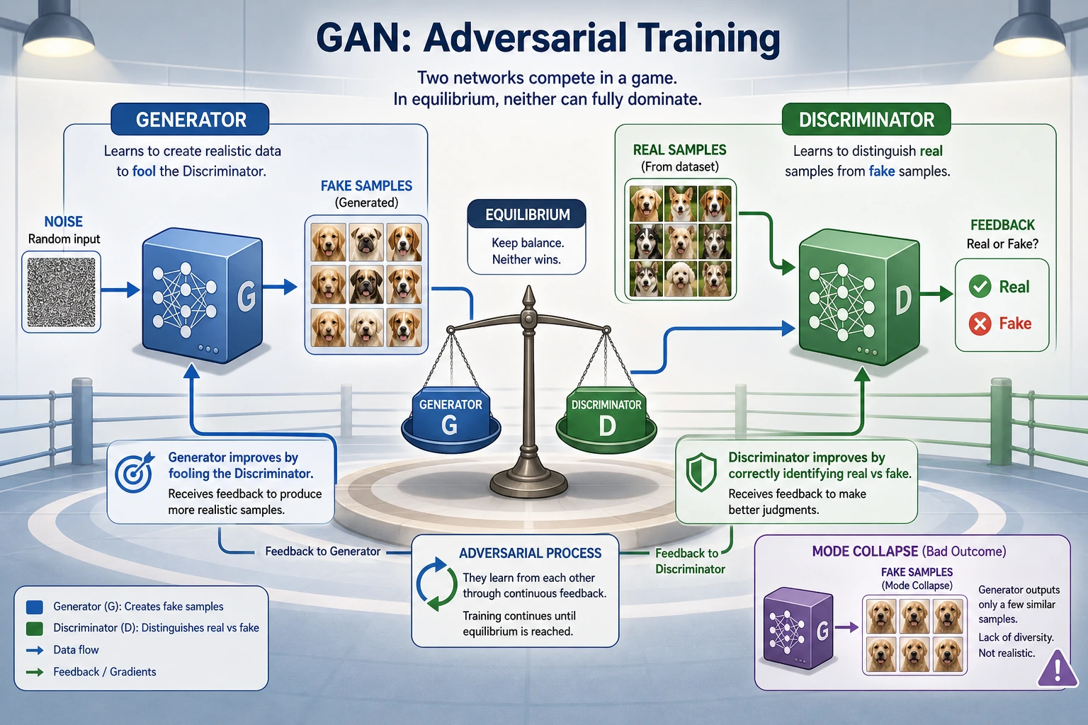
A GAN is a two-player training loop: the generator tries to create fake samples that look real, while the discriminator tries to tell real and fake apart. The power and the instability come from the same place: both players keep changing.

Learning Objectives

• Explain the roles of the generator and discriminator.
• Run a minimal PyTorch GAN on 1D data.
• Read loss_d, loss_g, fake_mean, and fake_std as training signals.
• Recognize mode collapse and discriminator/generator imbalance.
• Know when GAN is useful, and when diffusion or other generative methods may be a better default.

---

See the Game First

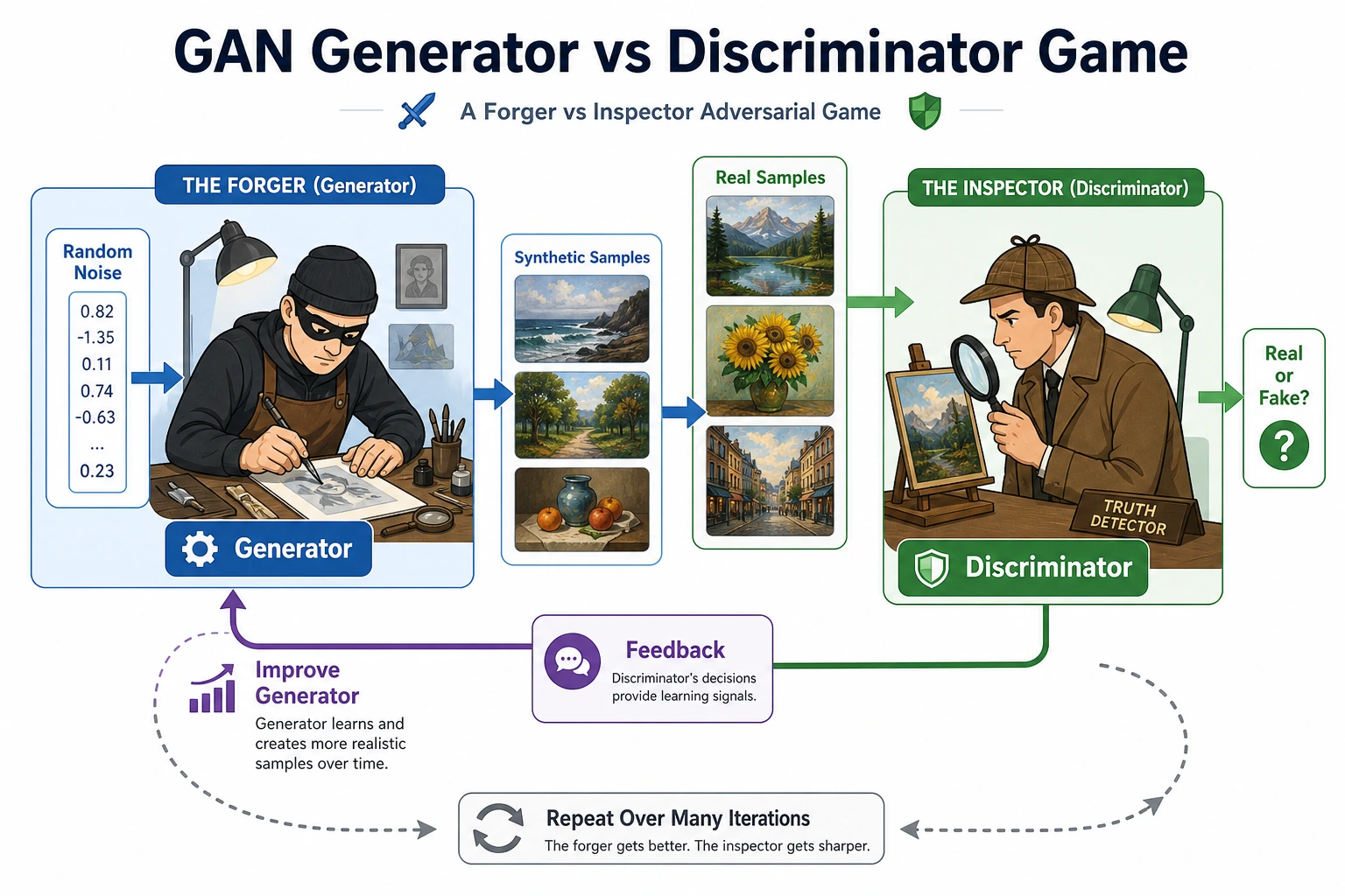
Part	Input	Output	Goal
Generator G	random noise z	fake sample	make fake look real
Discriminator D	real or fake sample	real/fake score	separate real from fake
Training loop	G and D updates	changing game	keep both sides learning

GAN is not trained with one fixed label target like ordinary classification. The discriminator changes what “hard to fool” means, and the generator changes what fake samples look like.

The Practical Loop

Read one GAN step as two updates:

1. Train D: real -> real, G(z).detach() -> fake
2. Train G: G(z) should make D say real

The .detach() in the discriminator step matters. It prevents the discriminator update from accidentally changing the generator.

Lab: Train a Tiny 1D GAN

This example does not generate images. It teaches the training mechanics with a real distribution centered near 2.0.

Create tiny_gan_1d.py:

import torch
from torch import nn

torch.manual_seed(7)


def real_batch(n):
    return torch.randn(n, 1) * 0.2 + 2.0


G = nn.Sequential(nn.Linear(2, 16), nn.ReLU(), nn.Linear(16, 1))
D = nn.Sequential(nn.Linear(1, 16), nn.ReLU(), nn.Linear(16, 1))

loss_fn = nn.BCEWithLogitsLoss()
opt_g = torch.optim.Adam(G.parameters(), lr=0.01)
opt_d = torch.optim.Adam(D.parameters(), lr=0.01)

for step in range(1, 301):
    real = real_batch(64)
    z = torch.randn(64, 2)
    fake = G(z).detach()

    d_real = D(real)
    d_fake = D(fake)
    loss_d = loss_fn(d_real, torch.ones_like(d_real)) + loss_fn(
        d_fake, torch.zeros_like(d_fake)
    )

    opt_d.zero_grad()
    loss_d.backward()
    opt_d.step()

    z = torch.randn(64, 2)
    fake = G(z)
    d_fake = D(fake)
    loss_g = loss_fn(d_fake, torch.ones_like(d_fake))

    opt_g.zero_grad()
    loss_g.backward()
    opt_g.step()

    if step in [1, 100, 200, 300]:
        with torch.no_grad():
            sample = G(torch.randn(256, 2))
            print(
                f"step={step:03d} "
                f"loss_d={loss_d.item():.3f} "
                f"loss_g={loss_g.item():.3f} "
                f"fake_mean={sample.mean().item():.3f} "
                f"fake_std={sample.std().item():.3f}"
            )

Run it:

python tiny_gan_1d.py

Expected output:

step=001 loss_d=1.579 loss_g=0.844 fake_mean=0.025 fake_std=0.117
step=100 loss_d=1.287 loss_g=0.654 fake_mean=1.093 fake_std=0.204
step=200 loss_d=1.460 loss_g=0.835 fake_mean=2.988 fake_std=0.291
step=300 loss_d=1.307 loss_g=0.630 fake_mean=1.384 fake_std=0.056

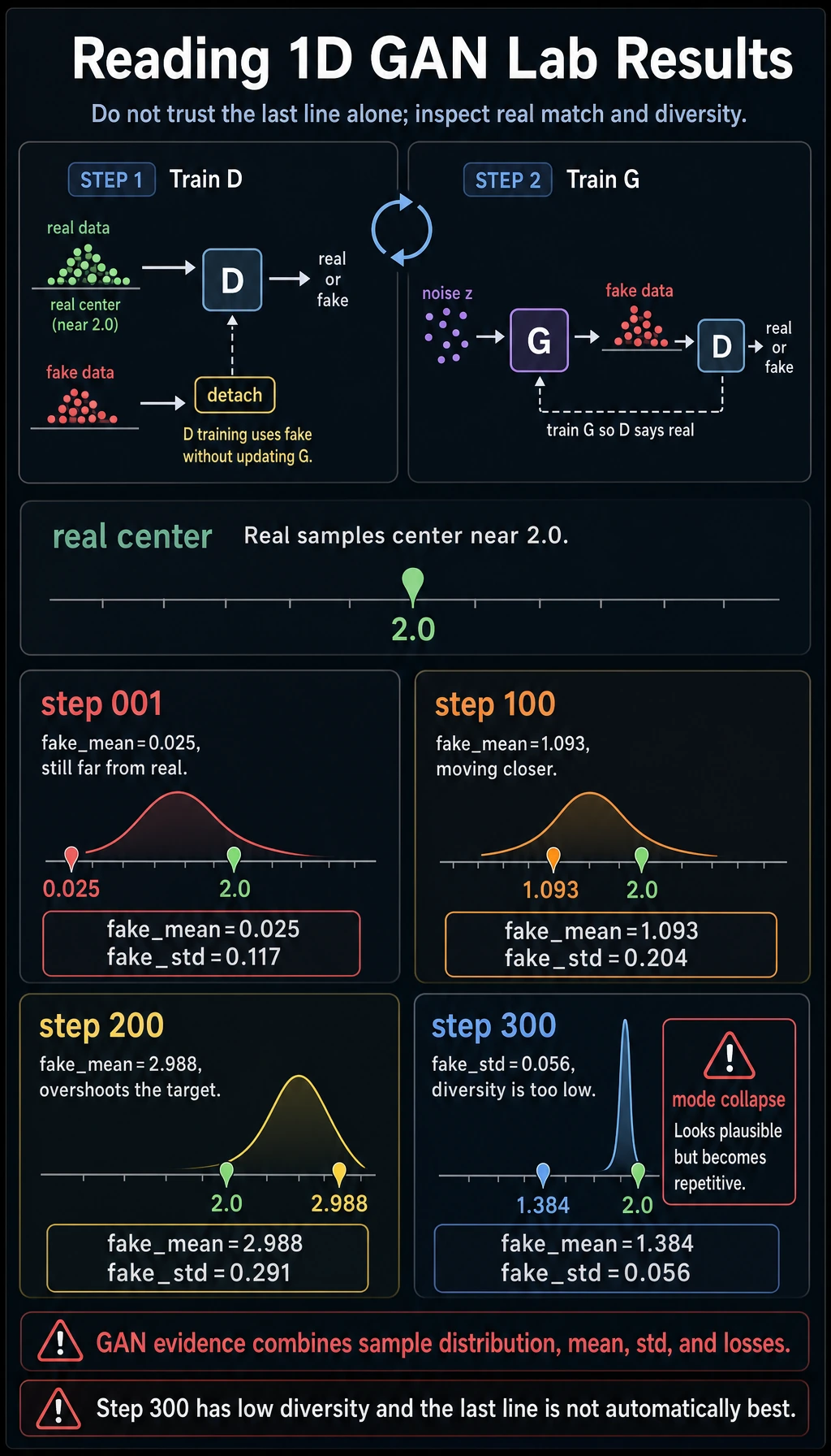
Do not read this as “the final line is best.” Read it as a diagnostic exercise:

• real samples are centered near 2.0;
• fake_mean moves around because G and D chase each other;
• fake_std becoming very small is a warning sign for low diversity;
• GAN loss curves can be hard to interpret without sample inspection.

What Is Mode Collapse?

Mode collapse means the generator finds one narrow trick that fools the discriminator, then keeps producing very similar samples.

In images, you may see many generated faces with nearly the same pose. In the 1D lab, a very small fake_std can be a simple collapse signal.

looks plausible but lacks diversity -> suspect mode collapse

Why GAN Training Is Hard

Problem	Symptom	First response
Discriminator too strong	G receives weak feedback	reduce D updates or capacity
Generator too weak	fake samples do not improve	tune learning rate, architecture, normalization
Mode collapse	samples become repetitive	monitor diversity, use stronger losses or regularization
Loss is misleading	loss changes but samples worsen	save sample grids and compare versions
Evaluation is fuzzy	“looks good” is subjective	combine visual checks with diversity and task metrics

When GAN Is Worth Learning

GAN is still worth learning because it teaches adversarial learning, distribution matching, and failure diagnostics very clearly.

For modern image generation projects, diffusion models are often more stable and easier to control. GAN remains especially useful when you want:

• fast sampling after training;
• adversarial realism signals;
• intuition about generated sample diversity;
• a concrete example of unstable multi-objective training.

Common Mistakes

Mistake	Fix
judging only by loss_g and loss_d	inspect generated samples and diversity
updating G during the D step	use G(z).detach()
letting D become perfect too early	tune capacity, update ratio, and learning rates
ignoring repeated outputs	track diversity and mode collapse
using GAN as the default for every generation task	compare with VAE, diffusion, or autoregressive methods

Exercises

1. Change the real data center from 2.0 to -1.0. Does fake_mean move?
2. Reduce lr from 0.01 to 0.001. Is training smoother or slower?
3. Increase the hidden size from 16 to 64. Does the game become more stable?
4. Print fake_std every 25 steps and mark possible collapse points.
5. Explain why GAN output quality cannot be judged from one loss number.

Key Takeaways

• GAN training is a moving two-player game.
• G learns to create samples, D learns to judge real vs fake.
• Instability is part of the training setup, not just a coding accident.
• Mode collapse means realism without diversity.
• GANs are valuable to understand, even when another generative family is the better production choice.