7.3.6 Model Scale and Computation

What this section is about

When many people talk about large models, they often focus on just one number:

• 7B
• 70B
• 671B

But when you actually train and deploy them, knowing the parameter count alone is nowhere near enough. You also need to look at:

• hidden size
• number of layers
• context length
• batch size
• KV cache
• throughput and latency

This lesson will break the vague phrase “the model is huge” into engineering language that you can actually calculate, estimate, and reason about.

Learning Objectives

• Understand the relationship between parameter scale, context length, and computational cost
• Understand why training and inference have different cost structures
• Learn how to make rough estimates of parameter count and KV cache with a runnable example
• Build a practical judgment of “why models cannot grow without limit”

---

Parameter Count Is Only the First Layer of the Story

Why do people like to say 7B / 70B?

Because it is intuitive. Parameter count does roughly reflect a model’s capacity:

• More parameters usually means a higher upper bound on expressive power

But that is only the first layer.

For large models, cost also depends on many other dimensions

For example, even if two models are both labeled 7B, they can still differ a lot because of factors like:

• different numbers of layers
• different hidden sizes
• different numbers of heads
• different context lengths
• whether they use GQA / MoE

So parameter count is not useless, but you cannot look at it alone.

An analogy: floor area is not the total cost of a building

You can think of parameter count as the total floor area of a house. But what really costs money also includes:

• building structure
• interior complexity
• heating and maintenance costs

Likewise, the real computational cost of a large model is not determined by parameter count alone.

---

Where Does the Parameter Count Come From?

In a decoder block, the main cost comes from attention and FFN

For a rough estimate, it helps to remember two main parts:

• Attention projection
• FFN projection

In many decoder-only models, the FFN can have even more parameters than attention.

A very useful rough formula

For a standard decoder block, you can use this approximate intuition:

• Attention-related parameters are about 4 * hidden^2
• FFN-related parameters are about 8 * hidden^2

So one layer can be roughly approximated as:

• 12 * hidden^2

Then multiply by the number of layers, and you get a very useful first-order estimate.

Why is a rough estimate still valuable?

Because engineering decisions do not need exact values down to the last digit at the beginning. What matters more is:

• the approximate order of magnitude
• which part is the main cost driver
• which hyperparameter change will raise cost most noticeably

---

Run a Truly Useful Estimation Script

The script below estimates two very common real-world things:

1. The approximate parameter count of a decoder-only model
2. The approximate KV cache usage during inference

def approx_decoder_params(num_layers, hidden_size, ffn_multiplier=4, vocab_size=50000):
    attention_params = 4 * hidden_size * hidden_size
    ffn_params = 2 * hidden_size * (hidden_size * ffn_multiplier)
    norm_params = 4 * hidden_size
    block_params = attention_params + ffn_params + norm_params
    embedding_params = vocab_size * hidden_size
    total = num_layers * block_params + embedding_params
    return total


def kv_cache_bytes(
    num_layers,
    seq_len,
    batch_size,
    num_kv_heads,
    head_dim,
    dtype_bytes=2,
):
    # 2 represents two caches: K and V
    return num_layers * batch_size * seq_len * num_kv_heads * head_dim * 2 * dtype_bytes


def human_readable(num_bytes):
    units = ["B", "KB", "MB", "GB", "TB"]
    value = float(num_bytes)
    for unit in units:
        if value < 1024 or unit == units[-1]:
            return f"{value:.2f} {unit}"
        value /= 1024


configs = [
    {
        "name": "small",
        "layers": 24,
        "hidden": 2048,
        "kv_heads": 16,
        "head_dim": 128,
        "seq_len": 4096,
    },
    {
        "name": "large",
        "layers": 48,
        "hidden": 4096,
        "kv_heads": 8,
        "head_dim": 128,
        "seq_len": 8192,
    },
]

for cfg in configs:
    params = approx_decoder_params(cfg["layers"], cfg["hidden"])
    kv_bytes = kv_cache_bytes(
        num_layers=cfg["layers"],
        seq_len=cfg["seq_len"],
        batch_size=1,
        num_kv_heads=cfg["kv_heads"],
        head_dim=cfg["head_dim"],
    )
    print("-" * 60)
    print("model       :", cfg["name"])
    print("rough params:", f"{params / 1e9:.2f}B")
    print("kv cache    :", human_readable(kv_bytes))

Expected output:

------------------------------------------------------------
model       : small
rough params: 1.31B
kv cache    : 768.00 MB
------------------------------------------------------------
model       : large
rough params: 9.87B
kv cache    : 1.50 GB

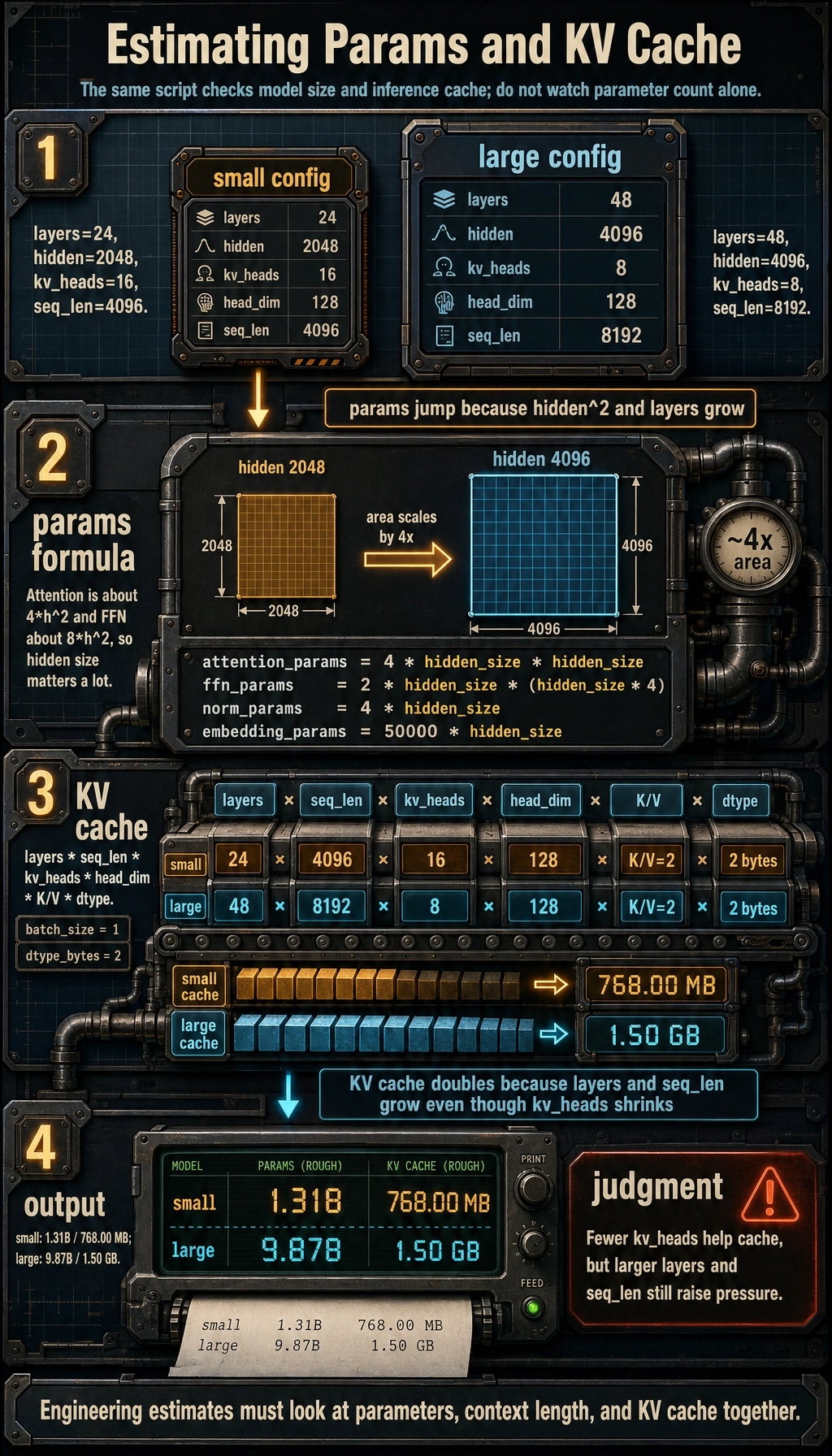
What is the most important takeaway from this code?

First:

• Parameter count is strongly related to hidden_size^2

That means once hidden size gets larger, cost increases very quickly.

Second:

• KV cache grows together with layers * seq_len * kv_heads * head_dim

This is why context length and inference memory affect each other.

Why is the pressure on the large model not just a doubling of parameters?

Because you will find that many factors are growing at the same time:

• more layers
• larger hidden size
• longer seq_len

Once these factors stack together, both training and inference costs rise significantly.

Why can GQA / MQA relieve inference pressure?

Because they directly reduce:

• num_kv_heads

And that is one of the core terms in the KV cache formula.

Reading the diagram

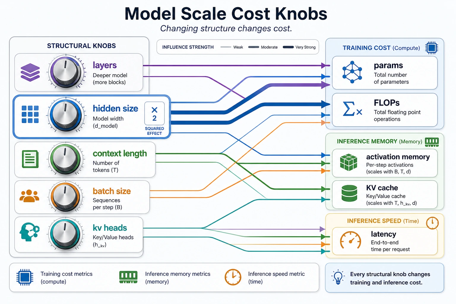
This diagram breaks cost into several knobs: layers, hidden size, context length, batch size, and kv heads. What beginners often underestimate is that these knobs multiply each other, especially hidden size, which usually affects both parameters and computation quadratically.

---

What Is Actually Different Between Training and Inference?

What usually becomes the bottleneck during training?

Common training bottlenecks include:

• model parameters
• gradients
• optimizer states
• intermediate activations

So during training, you will care a lot about:

• mixed precision
• gradient checkpointing
• tensor parallelism / data parallelism
• activation memory

What usually becomes the bottleneck during inference?

The main pressure during inference more often comes from:

• KV cache
• throughput
• latency per request
• GPU memory under concurrency

So you will care more about:

• how to set batch size
• how long the context is
• how many kv heads there are
• whether the cache can be quantized

Why does “the model can be trained” not mean “it is easy to deploy”?

Because training and inference are fundamentally different workloads.

Training is more like:

• large batches, continuous updates, throughput first

Inference is more like:

• real-time responses, cache accumulation, latency sensitive

That is why some model training setups are feasible, but deployment is still extremely painful.

Reading the diagram

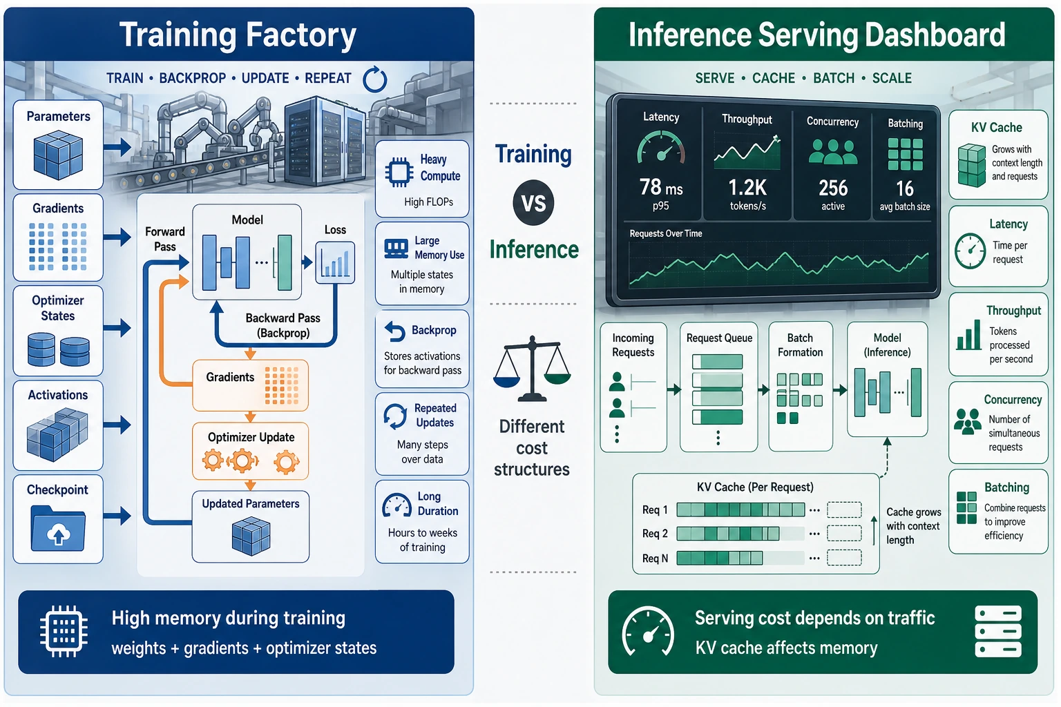
Training is more like “continuous production,” where the focus is on parameters, gradients, optimizer states, and intermediate activations. Inference is more like “real-time service,” where the focus is on KV cache, latency, throughput, and memory under concurrency. Being trainable does not mean being easy to deploy, because the bottlenecks on each side are completely different.

---

Scaling Is Not About Bigger Is Better, but About Bigger Is More Expensive

Parameter growth creates opportunities for capability, not free performance

More parameters usually bring a higher expressive ceiling, but only if you also have:

• enough data
• enough training tokens
• enough compute

Otherwise, the model is just “bigger,” not necessarily “more worthwhile.”

Longer context is not free either

Increasing context length brings:

• more usable information

But it also brings:

• higher attention cost
• larger KV cache
• harder long-range information utilization

So “supports 128k” does not mean “all 128k are necessarily useful.”

Three common real-world problems when scaling up

1. Training cost rises sharply
2. Inference service cost increases at the same time
3. If data and training tokens are insufficient, marginal gains decline

So the essence of scaling is:

• finding a balance among capability, cost, and data

---

A Very Practical Decision Order

If you are stuck on the training side

First check:

• Is hidden size too aggressive?
• Are batch size and seq_len too high?
• Are intermediate activations the main bottleneck?

If you are stuck on the inference side

First check:

• context length
• concurrency
• KV cache size
• whether you can use GQA / MQA / cache quantization

If you are planning model scale

First ask:

1. Can my data scale support it?
2. Can my training budget handle it?
3. Can I afford the inference cost after launch?

If you do not think about these three together, model planning easily turns into the illusion that “bigger is always better.”

---

Common Misconceptions

Misconception 1: If the parameter count is large, the result must be good

Not necessarily. Parameter count is only capacity, not automatically realized performance.

Misconception 2: Inference cost depends only on parameter count

Wrong. Context length and KV cache are often just as important.

Misconception 3: Training memory and inference memory are the same thing

No. Their memory composition and bottlenecks are different.

---

Summary

The most important thing in this lesson is not to memorize how many B some model has, but to build a more realistic language:

Model scale = parameter capacity, while computational cost is determined together by parameters, layers, hidden size, context length, KV cache, batch size, and engineering implementation.

Once you can look at all these factors together, you will truly gain an engineering intuition for why large models are expensive, where that expense comes from, and how to control it.

---

Exercises

1. Change seq_len in the example from 4096 to 16384, and observe how KV cache usage changes.
2. Why is hidden size often more “expensive” than many people expect?
3. Explain in your own words: why does a model being trainable not mean deployment will be easy?
4. If you want to build a long-context chat service, besides parameter count, what metrics would you care about first?