7.6.4 Other PEFT Methods [Optional]

Section overview

In the previous section, we already learned the main storyline of LoRA and QLoRA: instead of retraining the entire large model, we only train a small number of additional parameters.

But PEFT is not only LoRA. The real question is actually:

Where exactly do we want to place the “trainable capability” in the model?

• Put it on the input side, and it becomes Prompt Tuning
• Put it in the context prefix of each layer, and it becomes Prefix Tuning
• Put it in a small module between layers, and it becomes Adapter
• Put it on the scaling factors of intermediate activations, and it becomes IA3

This section organizes these branches into a map that you can really use for choosing an approach.

Learning objectives

• Understand where Prompt Tuning, Prefix Tuning, Adapter, and IA3 each make changes
• Know the core differences between these methods and LoRA
• Run a minimal Adapter training example that is truly related to the PEFT topic
• Build intuition for choosing methods in multi-task, low-memory, fast-switching scenarios

---

Why isn’t LoRA the only answer?

What PEFT is really trying to solve is not “inventing acronyms”

The core problem of PEFT is very simple:

If we freeze the main body of a large model and train only a very small part of the parameters, can we still adapt the model to a new task?

As long as this goal stays the same, “which small part of the parameters to train” will naturally lead to many variants.

So the biggest difference between these methods is not their names, but:

• Where the trainable parameters are placed
• Which part of the model’s information flow they affect
• How training cost, inference cost, and reusability compare

An analogy: making lightweight modifications to the same computer

You can think of a base model as a computer that is already assembled:

• Prompt Tuning is like putting a few hidden sticky notes on the desktop at startup
• Prefix Tuning is like preloading some context before each software starts
• Adapter is like plugging a tiny expansion card into the motherboard
• IA3 is like adding adjustable gain controls to a few key knobs

None of these rebuild the whole computer. They all add a layer of adjustable structure at different positions.

Why do real projects need these branches?

Because engineering constraints are not exactly the same:

• Some teams care most about memory usage
• Some care most about fast task switching
• Some care most about not slowing down inference
• Some want to attach many domain adapters to the same base model

Even though they are all PEFT, the best method may not be the same.

---

First, clarify the PEFT family map

Prompt Tuning: put the trainable part in front of the input

The intuition behind Prompt Tuning is:

Instead of changing the internal structure of the model, attach a small set of trainable “soft prompts” before the input embedding.

Here, the prompt is not natural language that you manually write, but a set of trainable vectors.

Its advantages are:

• Extremely few parameters
• Clear concept and easy to understand
• Suitable when there are many tasks and each task adaptation should be very light

Its limitations are:

• Limited ability to transform complex tasks
• Mainly affects the input side, not as deep as layer-level modifications

Prefix Tuning: add “prefix context” to each layer

Prefix Tuning goes one step further than Prompt Tuning.

Instead of adding vectors only at the very beginning of the input, it:

prepares an extra trainable key/value prefix for the attention module in each Transformer layer.

You can think of it like this:

• Prompt Tuning is more like inserting a sentence of “task instructions” at the beginning
• Prefix Tuning is like every layer can see an extra piece of contextual guidance when doing attention

So it usually has stronger expressiveness than Prompt Tuning.

Adapter: insert a small module between layers

Adapter is easy for beginners to understand because it is most like “explicitly adding a plugin.”

A common structure is:

1. The original hidden state first goes through a down-projection layer
2. A non-linear transformation is applied in the middle
3. Then it is projected back to the original dimension
4. It is added back to the main path through a residual connection

In other words:

Freeze the main path, and insert a tiny trainable side path next to it.

Its engineering advantages are very clear:

• No major changes to the original model body
• Different tasks can use different adapters
• When switching tasks, you only need to swap the small module

IA3: instead of learning a large matrix, learn “scaling coefficients”

The idea behind IA3 is even more restrained:

Instead of inserting a small network or learning a large increment, only learn a small number of per-channel scaling vectors.

For example, on attention outputs or feed-forward activations, it can:

• Amplify some dimensions
• Suppress some dimensions

This means:

• Fewer parameters
• Lighter training
• But also relatively more limited expressive power

Looking at the four methods together

Method	Where the trainable part is placed	Intuition	Common advantages	Common limitations
Prompt Tuning	Before the input embedding	Feed the model a soft prompt	Extremely few parameters	Limited transformation power
Prefix Tuning	KV prefix in each layer’s attention	Each layer sees extra context	More expressive than soft prompts	Higher implementation complexity
Adapter	Small bottleneck module between layers	Insert a lightweight plugin	Easy multi-task switching	Adds a little extra computation at inference
IA3	Activation scaling vector	Adjust the gain of key channels	Extremely few parameters, lightweight implementation	Weaker expressiveness for complex changes

Reading tip

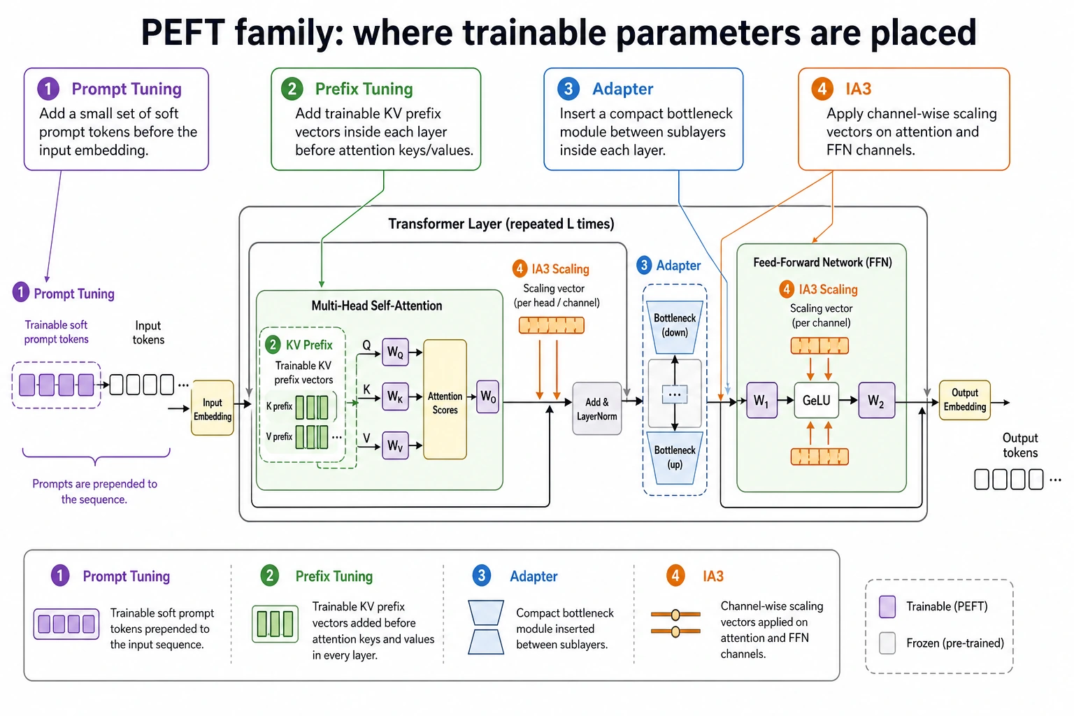
Don’t memorize this figure by method name. Focus on “where the trainable part is placed”: Prompt Tuning is before the input, Prefix Tuning is the KV prefix of attention in each layer, Adapter inserts a small module between layers, and IA3 adjusts channel scaling. Different locations mean different costs, expressive power, and switching behavior.

A small glossary for the PEFT family

Term	Beginner-friendly explanation
PEFT	Parameter-Efficient Fine-Tuning: adapt a model by training only a small part of the parameters
Soft prompt	Trainable vectors, not readable natural-language instructions
KV prefix	Extra trainable key/value vectors that attention can look at
Bottleneck	A small down-projection then up-projection module that limits parameter count
Residual connection	Add the small adaptation result back to the original hidden state
Activation scaling	Multiply some hidden dimensions by learned factors to amplify or suppress them

---

First, run a real Adapter example related to PEFT

The example below will do something very specific:

• Build a very small text classification task
• Freeze the base encoder
• Train only the Adapter and the classification head

This lets you directly see that:

• The main model is unchanged
• A small number of parameters can still learn the task

Run note

pip install torch

import torch
import torch.nn as nn

torch.manual_seed(42)

samples = [
    ("refund my order", 0),
    ("need a refund", 0),
    ("cancel and refund", 0),
    ("login failed again", 1),
    ("cannot login account", 1),
    ("password login problem", 1),
]
label_names = ["refund", "login"]

vocab = {"<pad>": 0}
for text, _ in samples:
    for token in text.split():
        if token not in vocab:
            vocab[token] = len(vocab)

max_len = max(len(text.split()) for text, _ in samples)


def encode(text):
    ids = [vocab[token] for token in text.split()]
    ids += [0] * (max_len - len(ids))
    return ids


x = torch.tensor([encode(text) for text, _ in samples], dtype=torch.long)
y = torch.tensor([label for _, label in samples], dtype=torch.long)


class FrozenBaseEncoder(nn.Module):
    def __init__(self, vocab_size, hidden_dim=16):
        super().__init__()
        self.embedding = nn.Embedding(vocab_size, hidden_dim)
        self.proj = nn.Linear(hidden_dim, hidden_dim)

        for param in self.parameters():
            param.requires_grad = False

    def forward(self, token_ids):
        emb = self.embedding(token_ids)
        mask = (token_ids != 0).unsqueeze(-1)
        pooled = (emb * mask).sum(dim=1) / mask.sum(dim=1).clamp(min=1)
        hidden = torch.tanh(self.proj(pooled))
        return hidden


class AdapterClassifier(nn.Module):
    def __init__(self, vocab_size, hidden_dim=16, bottleneck_dim=4, num_labels=2):
        super().__init__()
        self.base = FrozenBaseEncoder(vocab_size, hidden_dim)
        self.adapter_down = nn.Linear(hidden_dim, bottleneck_dim)
        self.adapter_up = nn.Linear(bottleneck_dim, hidden_dim)
        self.classifier = nn.Linear(hidden_dim, num_labels)

    def forward(self, token_ids):
        hidden = self.base(token_ids)
        adapted = hidden + self.adapter_up(torch.tanh(self.adapter_down(hidden)))
        logits = self.classifier(adapted)
        return logits


model = AdapterClassifier(vocab_size=len(vocab))
optimizer = torch.optim.Adam(
    [p for p in model.parameters() if p.requires_grad],
    lr=0.05,
)
criterion = nn.CrossEntropyLoss()

total_params = sum(p.numel() for p in model.parameters())
trainable_params = sum(p.numel() for p in model.parameters() if p.requires_grad)
print("total params     =", total_params)
print("trainable params =", trainable_params)

for step in range(201):
    logits = model(x)
    loss = criterion(logits, y)

    optimizer.zero_grad()
    loss.backward()
    optimizer.step()

    if step % 50 == 0:
        preds = logits.argmax(dim=-1)
        acc = (preds == y).float().mean().item()
        print(f"step={step:03d} loss={loss.item():.4f} acc={acc:.2f}")

with torch.no_grad():
    preds = model(x).argmax(dim=-1)
    for text, pred in zip([text for text, _ in samples], preds.tolist()):
        print(f"{text:22s} -> {label_names[pred]}")

Expected output:

total params     = 694
trainable params = 182
step=000 loss=0.7183 acc=0.50
step=050 loss=0.0000 acc=1.00
step=100 loss=0.0000 acc=1.00
step=150 loss=0.0000 acc=1.00
step=200 loss=0.0000 acc=1.00
refund my order        -> refund
need a refund          -> refund
cancel and refund      -> refund
login failed again     -> login
cannot login account   -> login
password login problem -> login

What exactly does this code teach?

It is not teaching you how to build a complete production-grade fine-tuning system. Instead, it deliberately focuses on Adapter itself:

• FrozenBaseEncoder is fully frozen
• adapter_down and adapter_up are newly added small modules
• classifier maps the adapted representation to labels

The truly key line is this:

adapted = hidden + self.adapter_up(torch.tanh(self.adapter_down(hidden)))

This is the classic Adapter idea:

• Keep the main representation
• Add a small bottleneck branch beside it
• Add it back in residual form

Why is this much better than “just printing the method name”?

Because now you can directly observe three things:

1. Only a very small part of the parameters is trainable
2. The main model does not change, yet the task can still be fit
3. The new capability comes from a small inserted module, not from retraining the whole network

These three points are the essence of Adapter.

---

Then look at three shorter structural illustrations

Prompt Tuning: concatenate soft prompts before the input

import torch

token_embeddings = torch.randn(1, 5, 8)
soft_prompt = torch.randn(1, 3, 8, requires_grad=True)

combined = torch.cat([soft_prompt, token_embeddings], dim=1)
print("Original length:", token_embeddings.shape[1])
print("Length after concatenation:", combined.shape[1])

Expected output:

Original length: 5
Length after concatenation: 8

The most important thing to remember here is:

• The soft prompt is not readable text
• It is a set of vectors learned during training
• What the model sees is the embedding of “extra input tokens”

Prefix Tuning: do not change the input length, change the context seen by attention in each layer

import torch

layer_keys = torch.randn(1, 4, 8)
prefix_keys = torch.randn(1, 2, 8, requires_grad=True)

all_keys = torch.cat([prefix_keys, layer_keys], dim=1)
print("Original number of attention keys:", layer_keys.shape[1])
print("Number of keys after adding prefix:", all_keys.shape[1])

Expected output:

Original number of attention keys: 4
Number of keys after adding prefix: 6

The intuition behind this illustration is:

• Normal attention only sees the original sequence
• Prefix Tuning lets each layer’s attention see an additional trainable prefix

IA3: instead of adding a module, multiply key channels by scaling factors

import torch

hidden = torch.tensor([[1.0, 2.0, 3.0, 4.0]])
gate = torch.tensor([0.5, 1.0, 1.5, 2.0], requires_grad=True)

scaled = hidden * gate
print("before:", hidden)
print("after :", scaled)

Expected output:

before: tensor([[1., 2., 3., 4.]])
after : tensor([[0.5000, 2.0000, 4.5000, 8.0000]], grad_fn=<MulBackward0>)

The core of IA3 is not “becoming more complex,” but “making lightweight adjustments only at the most important positions.”

Read the printouts as structure

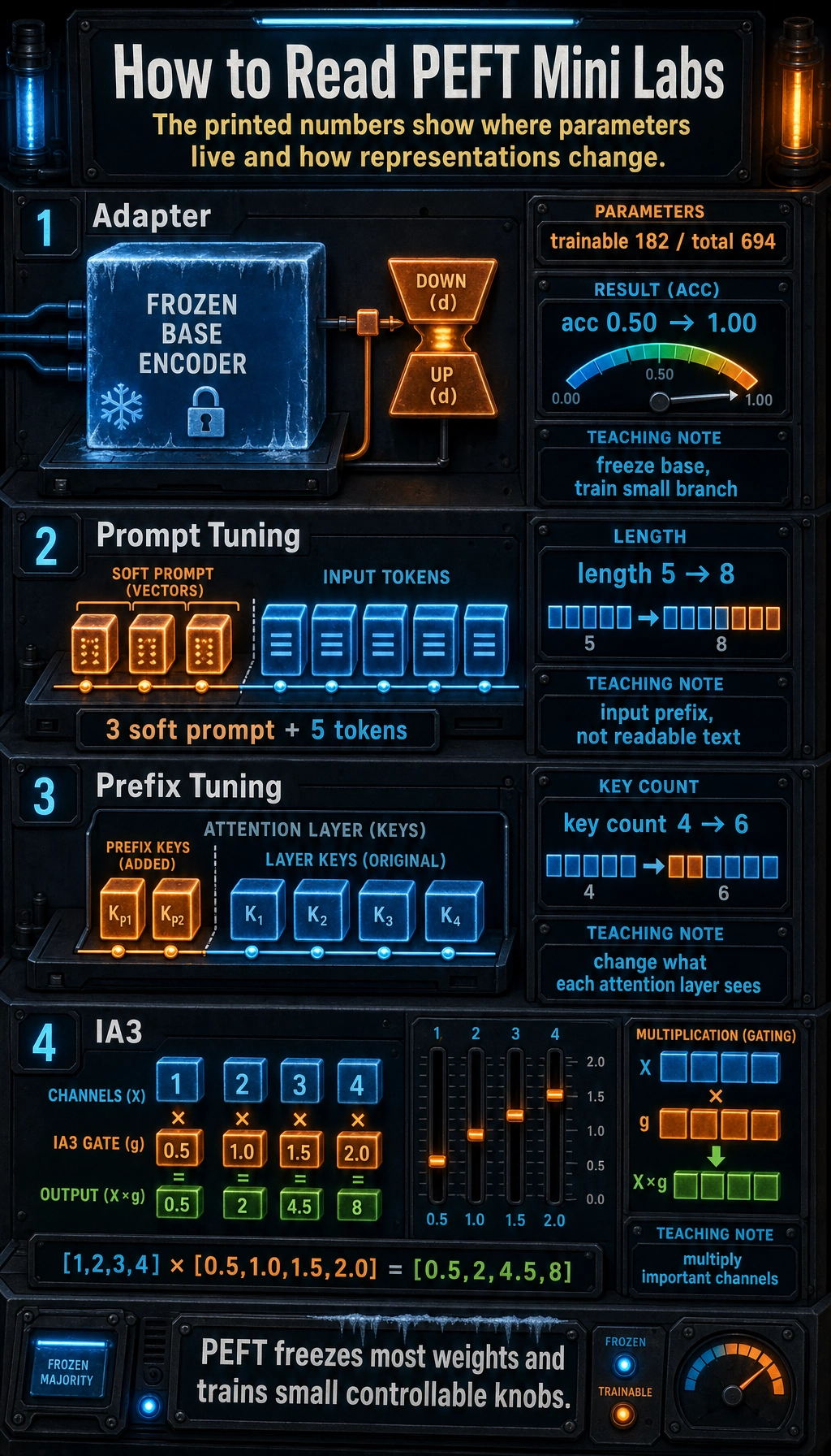
These short outputs are not just numbers. Adapter shows how few parameters move, Prompt Tuning changes input length, Prefix Tuning changes attention keys, and IA3 changes channel strength by multiplication.

---

How should you choose?

If you care most about task switching and modularity

Think first about:

• Adapter

Because it is naturally suitable for:

• One base model
• Many small adapters attached to it
• Loading different adapters for different tasks

If you care most about having even fewer parameters

You can first look at:

• Prompt Tuning
• IA3

These methods are very lightweight, but keep in mind:

• Fewer parameters does not automatically mean better results
• For complex tasks, expressive power may not be enough

If you want deeper intervention

You can look at:

• Prefix Tuning

Because it affects not only the very beginning of the input, but also how each layer’s attention reads context.

If you want a default industrial choice to try first

In practice, many teams still try:

• LoRA / QLoRA

The reason is simple:

• Mature ecosystem
• Rich tooling
• Lots of community experience

So this section is not asking you to abandon LoRA, but to let you know:

LoRA is only the most commonly used piece of the PEFT map, not the whole map.

---

These misconceptions are very common

Misconception 1: fewer parameters always means more advanced

Not necessarily. Fewer parameters mean:

• Cheaper training

But they can also mean:

• More limited expressive power

Misconception 2: the more method names you know, the more you understand

What you really need to know is:

• What does it change?
• Which part of the information flow does it affect?
• Why is it suitable for the current task?

Misconception 3: treating the “trainable module” as the only thing that matters

Don’t forget that success also depends heavily on:

• Data quality
• Prompt/template format
• Evaluation method
• Whether fine-tuning is really needed

---

Summary

What you should take away from this section is not the four names, but one main thread:

The essence of PEFT is to insert a small amount of trainable capability at an appropriate location, while changing the large model body as little as possible.

When you encounter a new PEFT variant later, you can also break it down with the same questions:

1. Where does it place the trainable parameters?
2. Does it affect the input, the inside of a layer, or the space between layers?
3. What engineering benefits does it bring, and what does it sacrifice?

Once these three things are clear, method names will no longer feel mysterious.

---

Exercises

1. Explain in your own words which part of the model Prompt Tuning, Prefix Tuning, Adapter, and IA3 each modify.
2. If you want to adapt one base model to 20 different business tasks at the same time, why is Adapter often attractive?
3. Change bottleneck_dim in the Adapter code in this section to a larger or smaller value, and observe how the number of trainable parameters changes.
4. Think about it: if your hardware is very limited but the task is fairly complex, which PEFT method would you try first? Why?