6.4.4 Sequence Modeling in Practice

Section Overview

This lesson turns sequence modeling into a small project: convert a continuous series into sliding-window samples, train an LSTM, compare against a naive baseline, and inspect validation predictions.

Learning Goals

• Convert a continuous time series into supervised learning samples.
• Keep LSTM inputs in [batch, seq_len, input_size].
• Split validation data in time order to avoid future leakage.
• Train an LSTM forecaster and compare it with a naive baseline.
• Read validation loss and prediction samples.

---

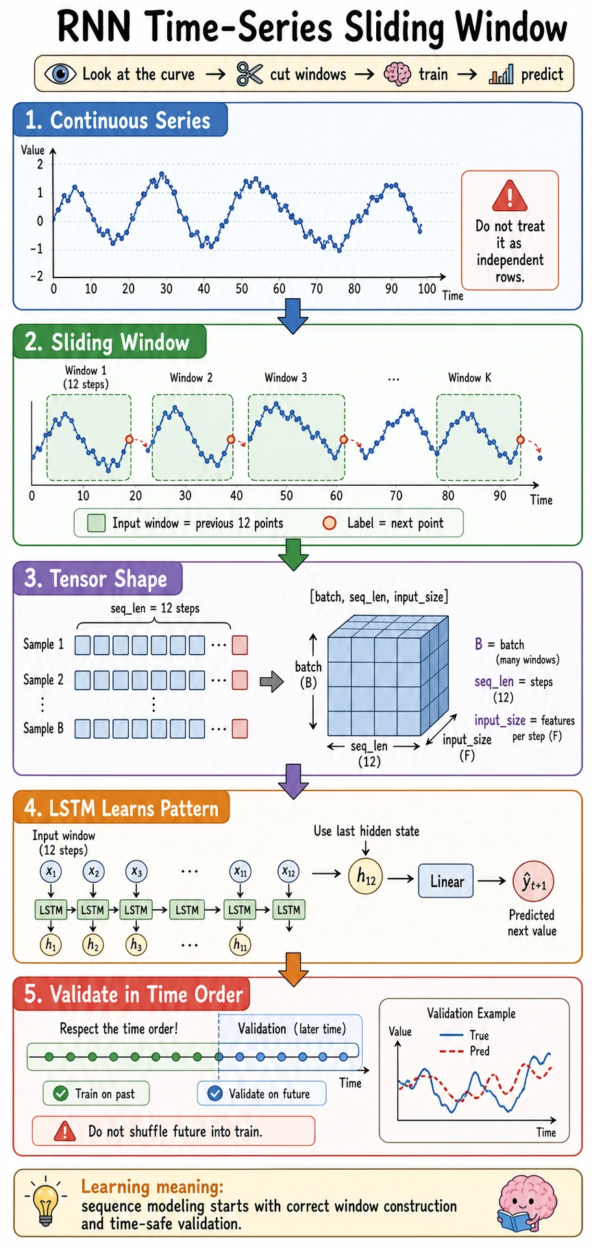
The Core Workflow

continuous series -> sliding windows -> time-order split -> LSTM -> validation MSE -> prediction inspection

For time series, avoid random splitting by default. If future points leak into training, validation becomes too optimistic.

Sliding Window in One Minute

If window_size = 3:

series: [1, 2, 3, 4, 5, 6]

X[0] = [1, 2, 3] -> y[0] = 4
X[1] = [2, 3, 4] -> y[1] = 5
X[2] = [3, 4, 5] -> y[2] = 6

That is how a continuous sequence becomes training rows.

Full Lab: LSTM Forecasting

The synthetic series combines two waves and noise. This is still small, but it is closer to real data than a perfect sine wave.

import numpy as np
import torch
from torch import nn

np.random.seed(42)
torch.manual_seed(42)


def make_windows(series, window_size):
    X, y = [], []
    for i in range(len(series) - window_size):
        X.append(series[i : i + window_size])
        y.append(series[i + window_size])
    X = torch.tensor(np.array(X), dtype=torch.float32).unsqueeze(-1)
    y = torch.tensor(np.array(y), dtype=torch.float32).unsqueeze(-1)
    return X, y


t = np.arange(0, 220)
series = (
    np.sin(t * 0.12)
    + 0.25 * np.sin(t * 0.03)
    + np.random.randn(len(t)) * 0.04
).astype(np.float32)

window_size = 16
X, y = make_windows(series, window_size)

split = int(len(X) * 0.8)
X_train, X_val = X[:split], X[split:]
y_train, y_val = y[:split], y[split:]

print("window_lab")
print("X:", tuple(X.shape), "y:", tuple(y.shape))
print("train:", tuple(X_train.shape), "val:", tuple(X_val.shape))

naive_val = ((X_val[:, -1, :] - y_val) ** 2).mean().item()
print("naive_val_mse:", round(naive_val, 4))


class LSTMForecaster(nn.Module):
    def __init__(self, hidden_size=32):
        super().__init__()
        self.lstm = nn.LSTM(1, hidden_size, batch_first=True)
        self.fc = nn.Linear(hidden_size, 1)

    def forward(self, x):
        out, _ = self.lstm(x)
        return self.fc(out[:, -1, :])


model = LSTMForecaster(32)
loss_fn = nn.MSELoss()
optimizer = torch.optim.Adam(model.parameters(), lr=0.01)

for epoch in range(1, 121):
    model.train()
    pred = model(X_train)
    loss = loss_fn(pred, y_train)

    optimizer.zero_grad()
    loss.backward()
    torch.nn.utils.clip_grad_norm_(model.parameters(), 1.0)
    optimizer.step()

    if epoch == 1 or epoch % 30 == 0:
        model.eval()
        with torch.no_grad():
            val_loss = loss_fn(model(X_val), y_val)
        print(f"epoch={epoch:03d} train_mse={loss.item():.4f} val_mse={val_loss.item():.4f}")

model.eval()
with torch.no_grad():
    val_pred = model(X_val)
    print("first_5_pred:", [round(v, 3) for v in val_pred[:5, 0].tolist()])
    print("first_5_true:", [round(v, 3) for v in y_val[:5, 0].tolist()])

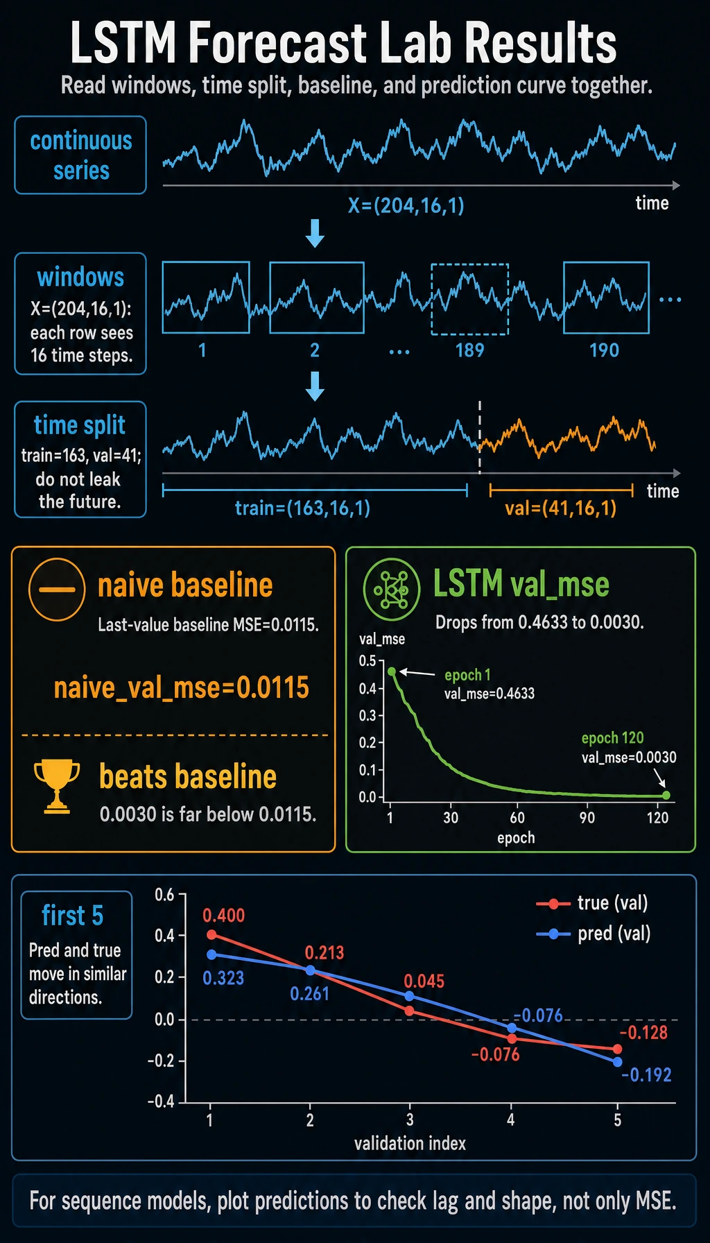
Expected output:

window_lab
X: (204, 16, 1) y: (204, 1)
train: (163, 16, 1) val: (41, 16, 1)
naive_val_mse: 0.0115
epoch=001 train_mse=0.5168 val_mse=0.4633
epoch=030 train_mse=0.0049 val_mse=0.0046
epoch=060 train_mse=0.0032 val_mse=0.0035
epoch=090 train_mse=0.0029 val_mse=0.0032
epoch=120 train_mse=0.0028 val_mse=0.0030
first_5_pred: [0.323, 0.261, 0.145, -0.025, -0.192]
first_5_true: [0.4, 0.213, 0.045, -0.076, -0.128]

Read the Output

Output	Meaning
X: (204, 16, 1)	204 windows, 16 time steps, 1 feature per step
train: (163, 16, 1)	first 80% of windows used for training
val: (41, 16, 1)	later windows used for validation
naive_val_mse	baseline: predict the next value as the last observed value
val_mse	LSTM validation error
first_5_pred vs first_5_true	quick sanity check for direction and scale

The LSTM beats the naive baseline in this run (0.0030 vs 0.0115). That matters: a model should beat a simple baseline before you trust it.

Why Use Gradient Clipping?

RNN-style models can sometimes produce large gradients. This line caps the total gradient norm:

torch.nn.utils.clip_grad_norm_(model.parameters(), 1.0)

It is not always required, but it is a good practical safety habit in sequence models.

What to Plot in a Notebook

In a notebook, add:

import matplotlib.pyplot as plt

plt.figure(figsize=(10, 4))
plt.plot(y_val.squeeze(-1).numpy(), label="true")
plt.plot(val_pred.squeeze(-1).numpy(), label="pred")
plt.legend()
plt.grid(True, alpha=0.3)
plt.show()

Look for:

• lag: predictions follow the shape but arrive late;
• flatline: model predicts an average value;
• missed peaks: window is too short or model too weak;
• noisy prediction: learning rate, data noise, or overfitting issues.

Common Pitfalls

Pitfall	Why it hurts	Fix
random train/val split	future leaks into training	split in time order
window too short	model cannot see enough context	try larger window_size
window too long	harder optimization, more noise	compare validation loss
no baseline	model may look good but be trivial	compare with naive last-value baseline
only checking MSE	trend may lag or flatten	plot prediction curves
no scaling on real data	large ranges destabilize training	normalize using train statistics

From Toy Series to Real Projects

Real sequence projects may use:

• multiple features per step;
• missing-value handling;
• normalization based only on training data;
• rolling-origin validation;
• GRU, Temporal CNN, Transformer, or statistical baselines;
• business metrics, not only MSE.

But the workflow stays the same: define windows, protect time order, compare baselines, and inspect predictions.

Exercises

1. Change window_size to 8 and 32. Which validation MSE is better?
2. Replace nn.LSTM with nn.GRU. Does it train faster or differently?
3. Remove gradient clipping. Does training remain stable?
4. Add a second feature, such as np.cos(t * 0.12).
5. Implement a rolling forecast that feeds predictions back into the next window.

Key Takeaways

• Sliding windows turn a continuous sequence into supervised learning samples.
• Time-based validation prevents future leakage.
• A naive baseline is required for meaningful evaluation.
• LSTM inputs use [batch, seq_len, input_size].
• Plots and prediction samples often reveal issues that a single loss value hides.