6.3.4 Classic CNN Architectures

Section Overview

Classic CNNs are useful when you read them as an engineering evolution, not as model-name trivia. Each generation fixed a real bottleneck: feasibility, scale, repeatable blocks, or trainable depth.

Learning Objectives

• Explain what LeNet, AlexNet, VGG, and ResNet each contributed.
• Read classic architectures by asking “what problem did this design solve?”
• Compare large kernels with stacked small kernels.
• Implement a minimal residual block.
• Decide what ideas still matter in modern CNN practice.

---

See the Evolution First

Read the timeline like this:

Architecture	What to remember	Main lesson
LeNet	early CNN skeleton	conv and pooling can recognize images
AlexNet	scale plus GPU training	deeper CNNs work when data, compute, and training tricks align
VGG	repeated 3 x 3 blocks	small kernels can build large receptive fields cleanly
ResNet	residual paths	very deep networks need easier gradient and information flow

The point is not to copy these models exactly today. The point is to inherit the design questions they answered.

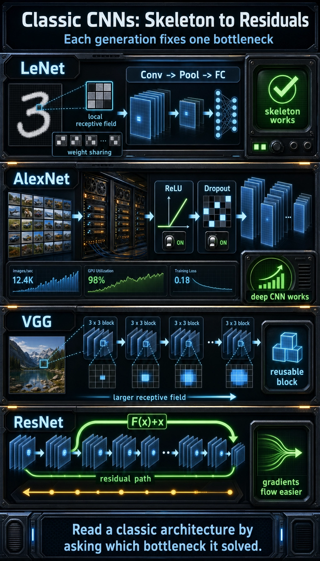
LeNet: The CNN Skeleton

LeNet is old, but the skeleton is still familiar:

Input -> Conv -> Pool -> Conv -> Pool -> Fully Connected -> Output

It taught three durable ideas:

• do not flatten images before extracting local patterns;
• use pooling to compress local responses;
• let later layers classify using higher-level features.

If you understand LeNet, you understand the minimum structure behind many image classifiers.

AlexNet: Scale Made CNNs Convincing

AlexNet mattered because it combined several forces at once:

• larger dataset;
• deeper CNN;
• GPU training;
• ReLU for faster optimization;
• Dropout for regularization.

Its lesson is practical: architecture alone rarely wins. Data, compute, training stability, and regularization all have to fit together.

For an experienced reader, this is the first systems lesson in CNN history: model quality is a stack, not a single clever layer.

VGG: Small Kernels, Repeated Blocks

VGG made a simple recipe popular:

Conv3x3 -> ReLU -> Conv3x3 -> ReLU -> Pool

Why stack small kernels instead of using one large kernel?

• stacked layers grow receptive field;
• each layer adds another nonlinearity;
• parameters can be more controlled;
• repeated blocks are easy to read and reproduce.

Lab 1: Compare Kernel Parameter Counts

This comparison is not the whole story, but it gives a useful intuition.

from torch import nn


def count_params(module):
    return sum(p.numel() for p in module.parameters() if p.requires_grad)


one_large_kernel = nn.Conv2d(16, 16, kernel_size=7, padding=3)
three_small_kernels = nn.Sequential(
    nn.Conv2d(16, 16, kernel_size=3, padding=1),
    nn.ReLU(),
    nn.Conv2d(16, 16, kernel_size=3, padding=1),
    nn.ReLU(),
    nn.Conv2d(16, 16, kernel_size=3, padding=1),
)

print("kernel_param_lab")
print("one 7x7 conv :", count_params(one_large_kernel))
print("three 3x3 conv:", count_params(three_small_kernels))

Expected output:

kernel_param_lab
one 7x7 conv : 12560
three 3x3 conv: 6960

The stacked 3 x 3 version has fewer parameters in this setup and adds nonlinear steps between convolutions. That is why VGG-style thinking became such a clean baseline.

Lab 2: Run a VGG-Style Block

import torch
from torch import nn

vgg_block = nn.Sequential(
    nn.Conv2d(3, 16, kernel_size=3, padding=1),
    nn.ReLU(),
    nn.Conv2d(16, 16, kernel_size=3, padding=1),
    nn.ReLU(),
    nn.MaxPool2d(2),
)

x = torch.randn(2, 3, 32, 32)
y = vgg_block(x)

print("vgg_block_lab")
print("input:", tuple(x.shape))
print("output:", tuple(y.shape))

Expected output:

vgg_block_lab
input: (2, 3, 32, 32)
output: (2, 16, 16, 16)

Read it as:

• two 3 x 3 convolutions refine features;
• pooling halves height and width;
• output channels become 16.

ResNet: Making Depth Trainable

A deeper network should be more expressive, but it can become harder to optimize. ResNet’s key idea is the residual connection:

output = learned_change(x) + x

Instead of forcing every block to learn a completely new representation, the block can learn a change on top of the input. If the block is not useful yet, the shortcut still carries information forward.

Lab 3: Implement a Residual Block

import torch
from torch import nn


class ResidualBlock(nn.Module):
    def __init__(self, channels):
        super().__init__()
        self.conv1 = nn.Conv2d(channels, channels, kernel_size=3, padding=1)
        self.relu = nn.ReLU()
        self.conv2 = nn.Conv2d(channels, channels, kernel_size=3, padding=1)

    def forward(self, x):
        identity = x
        out = self.relu(self.conv1(x))
        out = self.conv2(out)
        out = out + identity
        return self.relu(out)


block = ResidualBlock(8)
x = torch.randn(2, 8, 16, 16)
y = block(x)

print("residual_block_lab")
print("input:", tuple(x.shape))
print("output:", tuple(y.shape))

Expected output:

residual_block_lab
input: (2, 8, 16, 16)
output: (2, 8, 16, 16)

Read architecture labs through numbers

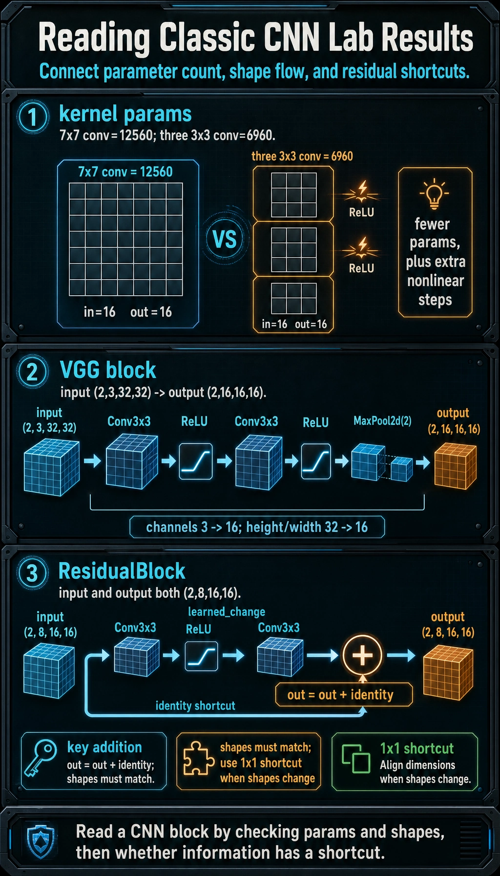
The three checks answer different questions: parameter count compares design cost, the VGG block shows how channels and spatial size change, and the residual block proves that the shortcut can only be added when shapes line up.

The most important line is:

out = out + identity

That addition is element-wise, so the shapes must match. Real ResNet variants use a 1 x 1 convolution in the shortcut when channel count or spatial size changes.

How to Read an Architecture Diagram

When you see a new CNN architecture, ask these questions:

Question	Why it matters
How does the first stage reduce spatial size?	too much early compression loses detail
Where do channels increase?	channels store feature diversity
Are blocks repeated?	repeated blocks make the architecture scalable
Is there a shortcut path?	shortcuts help optimization and information flow
How does the classifier head work?	Flatten and GAP have different parameter costs

This is more useful than memorizing exact layer counts.

What Still Matters Today?

You may not start a modern project from LeNet or AlexNet, but their ideas still show up:

• LeNet: the feature-extractor/classifier split;
• AlexNet: data, compute, activation, and regularization as a system;
• VGG: repeated simple blocks;
• ResNet: residual paths as a default design tool.

Modern CNN backbones and hybrid vision models still reuse these ideas, even when the names and blocks look newer.

Common Mistakes

Mistake	Better view
memorizing model names	remember the bottleneck each model solved
thinking VGG is only “many layers”	its real lesson is repeated small-kernel blocks
thinking ResNet is only “very deep”	its real lesson is making depth trainable
copying classic models directly	usually start from a pretrained modern backbone
ignoring compute cost	architecture choice must fit data size and deployment limits

Exercises

1. Summarize LeNet, AlexNet, VGG, and ResNet in one sentence each.
2. Change ResidualBlock(8) to ResidualBlock(16) and update the input tensor.
3. Remove one 3 x 3 convolution from the VGG-style block. What changes and what stays the same?
4. Explain why out + identity fails if channel counts differ.
5. Pick a modern CNN backbone and identify which classic ideas it still uses.

Key Takeaways

• Classic CNNs are a design evolution, not a name list.
• LeNet gave the skeleton; AlexNet proved scale; VGG made repeated small blocks clean; ResNet made depth easier to train.
• Stacked small kernels can be parameter-efficient and expressive.
• Residual connections preserve information and improve optimization.
• The practical skill is reading the design motivation behind an architecture.