6.3.6 CNN Practice: Image Classification

Section Overview

This is the “put it all together” lesson. You will create a small image dataset, train a CNN, validate it, inspect predictions, and decide what to try next.

Learning Objectives

• Build a complete image classification workflow.
• Keep image tensors in [N, C, H, W] format.
• Train and validate a CNN with CrossEntropyLoss.
• Inspect a confusion matrix and single-sample probabilities.
• Understand what changes when you move from this toy task to real images.

---

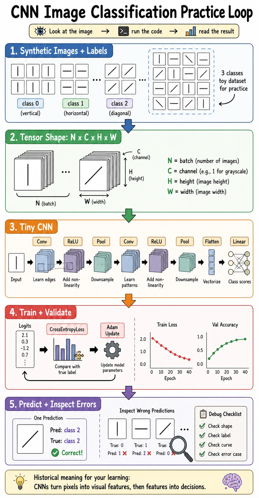
The Minimal Closed Loop

An image classification project needs:

images -> labels -> train/validation split -> CNN -> loss -> optimizer -> metrics -> error inspection

Do not skip validation or error inspection. A model that “runs” is not the same as a model that learned the right signal.

Full Lab: Train a Four-Class CNN

This lab uses four simple classes:

Label	Pattern
0	vertical line
1	horizontal line
2	diagonal down
3	diagonal up

Run the full script:

import numpy as np
import torch
from torch import nn

SEED = 42
np.random.seed(SEED)
torch.manual_seed(SEED)

CLASS_NAMES = ["vertical", "horizontal", "diag_down", "diag_up"]


def make_image(label, size=16, noise=0.08):
    img = np.zeros((size, size), dtype=np.float32)
    c = size // 2
    if label == 0:
        img[:, c] = 1.0
    elif label == 1:
        img[c, :] = 1.0
    elif label == 2:
        for i in range(size):
            img[i, i] = 1.0
    elif label == 3:
        for i in range(size):
            img[i, size - 1 - i] = 1.0

    img += np.random.randn(size, size).astype(np.float32) * noise
    return np.clip(img, 0.0, 1.0)


def make_dataset(per_class=120):
    X, y = [], []
    for label in range(len(CLASS_NAMES)):
        for _ in range(per_class):
            X.append(make_image(label))
            y.append(label)

    X = np.array(X, dtype=np.float32)
    y = np.array(y, dtype=np.int64)
    idx = np.random.permutation(len(X))
    X = torch.tensor(X[idx]).unsqueeze(1)
    y = torch.tensor(y[idx])
    split = int(len(X) * 0.8)
    return X[:split], y[:split], X[split:], y[split:]


class TinyCNNClassifier(nn.Module):
    def __init__(self, num_classes=4):
        super().__init__()
        self.features = nn.Sequential(
            nn.Conv2d(1, 8, kernel_size=3, padding=1),
            nn.ReLU(),
            nn.MaxPool2d(2),
            nn.Conv2d(8, 16, kernel_size=3, padding=1),
            nn.ReLU(),
            nn.MaxPool2d(2),
            nn.Conv2d(16, 32, kernel_size=3, padding=1),
            nn.ReLU(),
            nn.AdaptiveAvgPool2d((1, 1)),
        )
        self.head = nn.Linear(32, num_classes)

    def forward(self, x):
        x = self.features(x)
        x = x.flatten(1)
        return self.head(x)


def accuracy(logits, y):
    return (logits.argmax(dim=1) == y).float().mean().item()


def confusion_matrix(pred, y, num_classes):
    matrix = torch.zeros(num_classes, num_classes, dtype=torch.int64)
    for true_label, pred_label in zip(y, pred):
        matrix[true_label, pred_label] += 1
    return matrix


X_train, y_train, X_val, y_val = make_dataset()
print("data_lab")
print("train:", tuple(X_train.shape), tuple(y_train.shape))
print("val  :", tuple(X_val.shape), tuple(y_val.shape))

model = TinyCNNClassifier(num_classes=len(CLASS_NAMES))
with torch.no_grad():
    z = X_train[:4]
    print("shape_lab")
    print("input:", tuple(z.shape))
    print("features:", tuple(model.features(z).shape))
    print("logits:", tuple(model(z).shape))

loss_fn = nn.CrossEntropyLoss()
optimizer = torch.optim.Adam(model.parameters(), lr=0.01)

for epoch in range(1, 81):
    model.train()
    train_logits = model(X_train)
    train_loss = loss_fn(train_logits, y_train)

    optimizer.zero_grad()
    train_loss.backward()
    optimizer.step()

    if epoch == 1 or epoch % 20 == 0:
        model.eval()
        with torch.no_grad():
            val_logits = model(X_val)
            val_loss = loss_fn(val_logits, y_val)
        print(
            f"epoch={epoch:02d} "
            f"train_loss={train_loss.item():.4f} "
            f"val_loss={val_loss.item():.4f} "
            f"train_acc={accuracy(train_logits, y_train):.3f} "
            f"val_acc={accuracy(val_logits, y_val):.3f}"
        )

model.eval()
with torch.no_grad():
    val_logits = model(X_val)
    val_pred = val_logits.argmax(dim=1)
    cm = confusion_matrix(val_pred, y_val, len(CLASS_NAMES))
    probs = torch.softmax(val_logits[0], dim=0)

print("confusion_matrix rows=true cols=pred")
print(cm)
print("sample_prediction")
print("true:", CLASS_NAMES[y_val[0].item()])
print("pred:", CLASS_NAMES[val_pred[0].item()])
print("probs:", [round(v, 3) for v in probs.tolist()])

Expected output:

data_lab
train: (384, 1, 16, 16) (384,)
val  : (96, 1, 16, 16) (96,)
shape_lab
input: (4, 1, 16, 16)
features: (4, 32, 1, 1)
logits: (4, 4)
epoch=01 train_loss=1.3883 val_loss=1.3776 train_acc=0.245 val_acc=0.188
epoch=20 train_loss=0.0193 val_loss=0.0080 train_acc=1.000 val_acc=1.000
epoch=40 train_loss=0.0000 val_loss=0.0000 train_acc=1.000 val_acc=1.000
epoch=60 train_loss=0.0000 val_loss=0.0000 train_acc=1.000 val_acc=1.000
epoch=80 train_loss=0.0000 val_loss=0.0000 train_acc=1.000 val_acc=1.000
confusion_matrix rows=true cols=pred
tensor([[30,  0,  0,  0],
        [ 0, 22,  0,  0],
        [ 0,  0, 18,  0],
        [ 0,  0,  0, 26]])
sample_prediction
true: vertical
pred: vertical
probs: [1.0, 0.0, 0.0, 0.0]

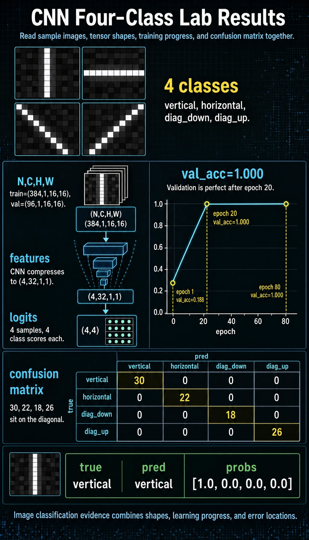
Read the Output

Output	Meaning
train: (384, 1, 16, 16)	384 grayscale training images
features: (4, 32, 1, 1)	CNN has compressed each image into 32 feature values
logits: (4, 4)	four samples, four class scores each
val_acc=1.000	the model learned this simple validation set
confusion matrix diagonal	true class and predicted class match

The confusion matrix is read row by row: rows are true labels, columns are predicted labels. Off-diagonal numbers are mistakes.

Why Use GAP Here?

The model uses AdaptiveAvgPool2d((1, 1)), also called Global Average Pooling in this context. It turns [N, 32, H, W] into [N, 32, 1, 1].

This keeps the classifier head small:

[N, 32, 1, 1] -> flatten -> [N, 32] -> Linear(32, 4)

For this lesson, GAP also avoids fragile manual calculations such as 16 * 3 * 3.

How to Diagnose Results

Symptom	Likely cause	Next action
train and val are both poor	model too weak, bad labels, LR issue	print shapes, inspect samples, adjust LR
train good but val poor	overfitting or split mismatch	add data, augmentation, regularization
loss does not move	wrong labels, no gradients, LR too small	check loss.backward(), labels, trainable params
high confidence wrong predictions	biased data or leakage in patterns	inspect examples and class distribution
only one class predicted	class imbalance or optimizer issue	print class counts and logits

From Toy Task to Real Images

This lesson intentionally keeps the dataset small and synthetic. Real projects add:

• Dataset and DataLoader;
• image file reading;
• train/validation/test split by source;
• data augmentation;
• pretrained backbone or transfer learning;
• model checkpointing;
• richer metrics such as precision, recall, and per-class accuracy.

The workflow is the same. The tooling becomes more serious.

Common Mistakes

Mistake	Fix
checking only training loss	always compute validation metrics
forgetting channel dimension	use [N, C, H, W]
using softmax before CrossEntropyLoss	pass raw logits to CrossEntropyLoss
ignoring wrong examples	inspect the confusion matrix and samples
making validation too similar to training	split by source when real images share context

Exercises

1. Increase noise from 0.08 to 0.25. How do validation results change?
2. Reduce per_class from 120 to 10. Does the model still generalize?
3. Remove AdaptiveAvgPool2d and use a Flatten head. What shape must Linear expect?
4. Add one more class, such as a square border.
5. Print the first five wrong validation examples if any exist.

Key Takeaways

• A complete image classification loop includes data, labels, split, model, loss, metrics, and error inspection.
• CNN inputs in PyTorch use [N, C, H, W].
• CrossEntropyLoss expects logits, not probabilities.
• GAP keeps the classifier head compact and shape-safe.
• Validation and error analysis are part of the model, not an afterthought.