6.2.3 PyTorch の基礎

この節の位置づけ

このページは API 一覧ではありません。目的は、PyTorch モデルを書く前に毎回必要になる反射を作ることです。学習前に shape、dtype、device、演算の意味を読む。

学習目標

• Python と NumPy のデータからテンソルを作れる。
• shape、dtype、device、各次元の意味を読める。
• 要素ごとの演算と行列積を区別できる。
• broadcasting を偶然ではなく意図して使える。
• 小さな順伝播を実行し、logits、確率、予測、loss を得られる。

---

まず Tensor のライフサイクルを見る

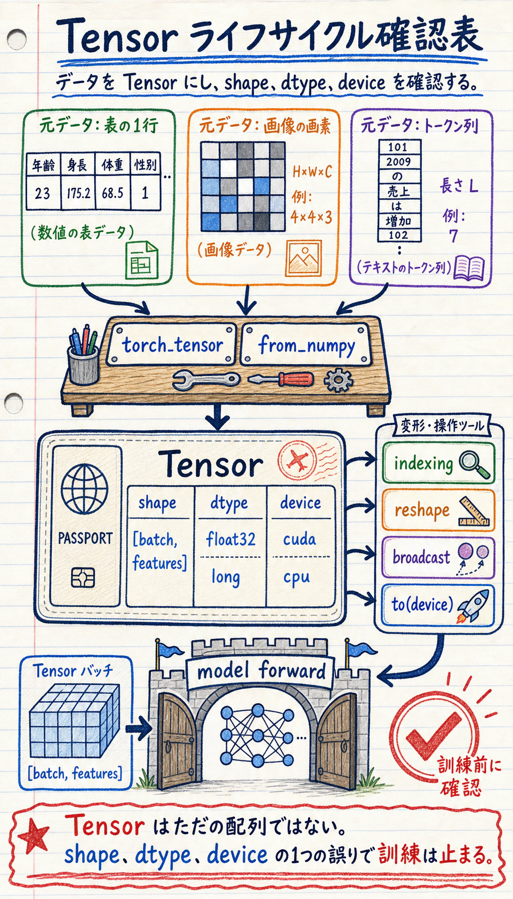
多くの PyTorch データは、次の流れを通ります。

生データ→tensor→shape/dtype/device の確認→演算/モデル→loss→勾配/更新

初心者がやりがちなのは、すぐモデルへ進むことです。より安全なのは、モデルに入れる前にテンソルを確認する習慣です。

Tensor は学習用の情報を持つデータ

短く実用的に言うと、次のようになります。

テンソルは、PyTorch が計算でき、device 間を移動でき、必要なら勾配も追跡できる多次元配列です。

NumPy 配列と比べると、PyTorch テンソルには深層学習向けの機能が 2 つあります。

• device: テンソルを CPU、GPU、Apple MPS に置ける。
• requires_grad: 自動微分に参加できる。

よく見る shape：

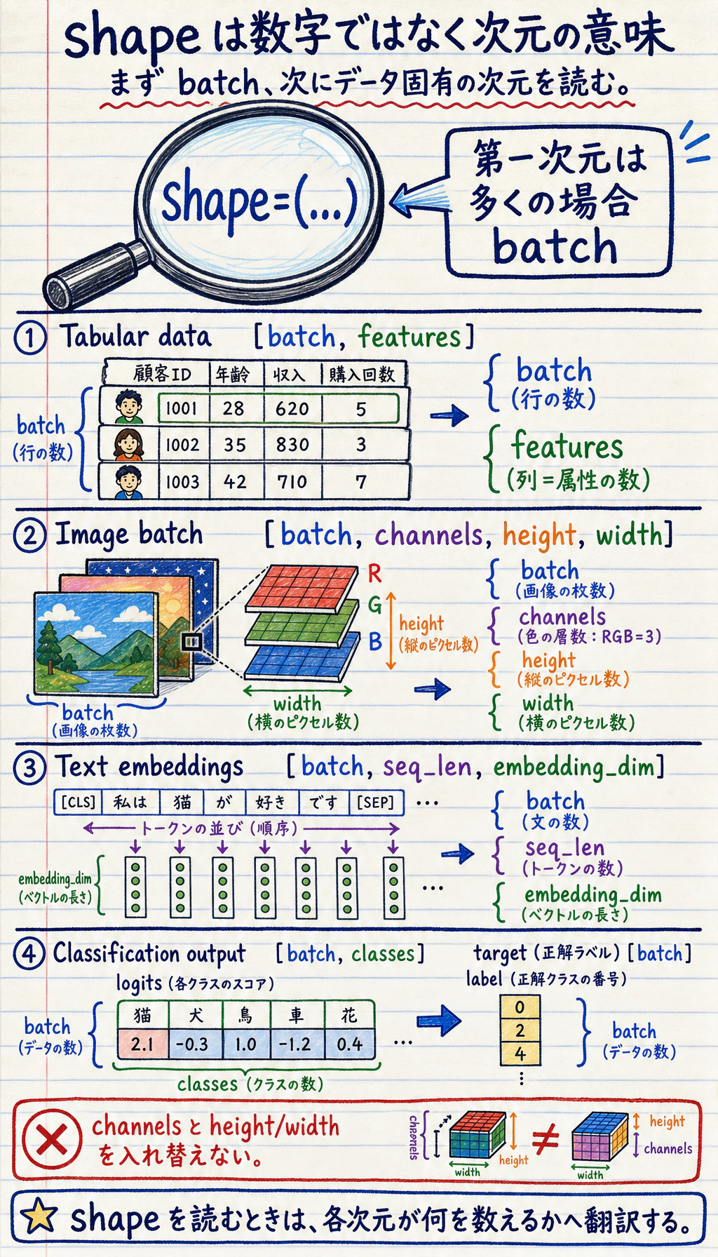
データ	よくある shape	意味
表形式の batch	[batch, features]	行がサンプル、列が特徴量
分類ラベル	[batch]	各サンプルに 1 つの整数クラス id
画像 batch	[batch, channels, height, width]	PyTorch の画像の慣例
テキスト埋め込み	[batch, seq_len, embedding_dim]	token ごとのベクトル表現
logits	[batch, classes]	softmax 前の生のクラススコア

実験 1: 計算する前にテンソルを調べる

まずこれを実行します。以後の学習ループで毎回使う確認習慣を作ります。

import torch


def describe(name, tensor, meaning):
    print(
        f"{name}: shape={tuple(tensor.shape)} "
        f"dtype={tensor.dtype} "
        f"device={tensor.device} "
        f"meaning={meaning}"
    )


X = torch.tensor(
    [
        [1.0, 2.0, 3.0],
        [4.0, 5.0, 6.0],
    ]
)
y = torch.tensor([0, 1], dtype=torch.long)

describe("X", X, "[batch, features]")
describe("y", y, "[batch]")

print("ndim:", X.ndim)
print("numel:", X.numel())
print("first row:", X[0])
print("feature means:", X.mean(dim=0))

期待される出力：

X: shape=(2, 3) dtype=torch.float32 device=cpu meaning=[batch, features]
y: shape=(2,) dtype=torch.int64 device=cpu meaning=[batch]
ndim: 2
numel: 6
first row: tensor([1., 2., 3.])
feature means: tensor([2.5000, 3.5000, 4.5000])

見るポイント：

• X は float32 で、通常のモデル入力によく使う型です。
• y は int64、つまり torch.long で、CrossEntropyLoss が分類ラベルに期待する型です。
• dim=0 は batch 方向に集約し、特徴量ごとの平均を返します。

実験 2: 特徴量から logits へ

次に、とても小さな分類用の順伝播を手で書きます。これは nn.Linear が内部でしていることに近いです。

import torch
import torch.nn as nn


def describe(name, tensor, meaning):
    print(
        f"{name}: shape={tuple(tensor.shape)} "
        f"dtype={tensor.dtype} "
        f"device={tensor.device} "
        f"meaning={meaning}"
    )


X = torch.tensor(
    [
        [1.0, 2.0, 3.0],
        [4.0, 5.0, 6.0],
    ]
)
y = torch.tensor([0, 1], dtype=torch.long)

W = torch.tensor(
    [
        [0.1, 0.2],
        [0.3, -0.1],
        [0.5, 0.4],
    ]
)
b = torch.tensor([0.01, -0.02])

logits = X @ W + b
probs = torch.softmax(logits, dim=1)
pred = probs.argmax(dim=1)
loss = nn.CrossEntropyLoss()(logits, y)

describe("logits", logits, "[batch, classes]")
print("logits:", torch.round(logits * 100) / 100)
print("probabilities:", torch.round(probs * 1000) / 1000)
print("prediction:", pred)
print("loss:", round(loss.item(), 3))

期待される出力：

logits: shape=(2, 2) dtype=torch.float32 device=cpu meaning=[batch, classes]
logits: tensor([[2.2100, 1.1800],
        [4.9100, 2.6800]])
probabilities: tensor([[0.7370, 0.2630],
        [0.9030, 0.0970]])
prediction: tensor([0, 0])
loss: 1.319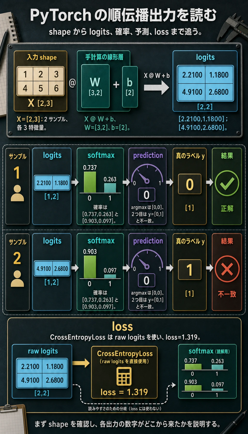

shape を丁寧に読みます。

• X は [2, 3]：2 サンプル、3 特徴量です。
• W は [3, 2]：3 入力特徴量、2 出力クラスです。
• X @ W は [2, 2]：各サンプルに 1 つのスコアベクトルです。
• b は [2] で、batch 全体へ broadcast されます。
• CrossEntropyLoss は softmax 後の確率ではなく、生の logits を受け取ります。

重要

PyTorch の多クラス分類では、生の logits を nn.CrossEntropyLoss() に渡します。loss の前に手動で softmax しないでください。softmax は、確率を読みたいときや予測を説明したいときに使います。

実際によく使う shape 操作

reshape、unsqueeze、squeeze を使って、次の演算が期待する shape に合わせます。

import torch

x = torch.arange(12)
grid = x.reshape(3, 4)
batch = grid.unsqueeze(0)
restored = batch.squeeze(0)

print("x:", tuple(x.shape))
print("grid:", tuple(grid.shape))
print("batch:", tuple(batch.shape))
print("restored:", tuple(restored.shape))

期待される出力：

x: (12,)
grid: (3, 4)
batch: (1, 3, 4)
restored: (3, 4)

実用的な意味：

• reshape(3, 4)：同じ 12 個の要素を表の形に並べ替える。
• unsqueeze(0)：batch 次元を追加する。
• squeeze(0)：サイズ 1 の batch 次元を取り除く。

view を使う理由がはっきり分かっている場合を除き、まずは reshape を使います。メモリ配置が連続でないときも、reshape のほうが扱いやすいです。

Broadcasting: 便利だが方向を確認する

Broadcasting とは、shape に互換性があるとき、小さいテンソルを大きいテンソルに合わせて自動的に拡張する仕組みです。

import torch

X = torch.tensor(
    [
        [1.0, 2.0, 3.0],
        [4.0, 5.0, 6.0],
    ]
)

feature_mean = X.mean(dim=0)
centered = X - feature_mean

print("feature_mean:", feature_mean)
print("centered:", centered)

期待される出力：

feature_mean: tensor([2.5000, 3.5000, 4.5000])
centered: tensor([[-1.5000, -1.5000, -1.5000],
        [ 1.5000,  1.5000,  1.5000]])

ここでは feature_mean の shape は [3]、X の shape は [2, 3] です。PyTorch は同じ特徴量平均を各行から引きます。

broadcasting に頼る前に、shape をコードのそばに書きます。

# X: [batch, features]
# feature_mean: [features]
centered = X - feature_mean

この小さなメモで、多くの静かな論理バグを防げます。

Device と NumPy 変換

実際の学習コードでは、テンソルを同じ device に置く必要があります。次の書き方なら CPU、CUDA、Apple Silicon MPS に対応できます。

import torch

if torch.cuda.is_available():
    device = torch.device("cuda")
elif torch.backends.mps.is_available():
    device = torch.device("mps")
else:
    device = torch.device("cpu")

X = torch.tensor([[1.0, 2.0, 3.0]])
X = X.to(device)

print("device:", X.device)

可視化や分析のために NumPy へ戻すときは、先に detach し、CPU へ移します。

arr = X.detach().cpu().numpy()
print(type(arr), arr.shape)

この順番が大事な理由：

• .detach() は勾配グラフから外します。
• .cpu() は NumPy がデータを読める場所に移します。
• .numpy() は NumPy 配列に変換します。

よくあるエラーパターン

症状	ありがちな原因	直し方
mat1 and mat2 shapes cannot be multiplied	行列積の次元が合わない	@ や nn.Linear の前に両方の shape を表示する
expected scalar type Long	分類 loss のラベルが float	y = y.long() を使う
Expected all tensors to be on the same device	モデルとデータが別 device にある	モデルとデータの両方を .to(device) する
loss は動くが結果がおかしい	broadcasting が想定外の方向に起きている	両方の shape を書き、拡張方向を確認する
NumPy 変換が失敗する	テンソルが GPU 上、または勾配グラフにつながっている	tensor.detach().cpu().numpy() を使う

クイックデバッグチェックリスト

テンソルをモデルへ入れる前に、まず表示します。

print("shape:", tuple(X.shape))
print("dtype:", X.dtype)
print("device:", X.device)
print("meaning: [batch, features]")

loss 関数の前には、これを確認します。

print("logits:", tuple(logits.shape), logits.dtype)
print("labels:", tuple(y.shape), y.dtype)

多クラス分類でよくある組み合わせは次です。

logits: [batch, classes], float32
labels: [batch], int64 / long

残す証拠

次へ進む前に、小さな tensor 点検メモを保存します。

入力形状

[batch, features]

logits 形状

[batch, classes]

ラベル形状

[batch]

ラベル型

CrossEntropyLoss に対して torch.long

デバイス確認

モデルとデータが同じデバイス上にある

これは後の PyTorch コードを最速でデバッグする方法です。初期の多くのエラーは、長い stack trace の中に隠れた shape、dtype、device、broadcasting の問題です。

練習

1. 実験 2 の X を 2 サンプルから 3 サンプルに変えてください。どの shape が変わり、どの shape は変わりませんか？
2. shape が [batch, 1] のラベルを作り、squeeze(1) で CrossEntropyLoss が受け取れる形に直してください。
3. X、W、b を device に移してください。1 つだけ移すとどんなエラーになりますか？
4. X @ W を X * W に変えてください。なぜ失敗する、または意味がまったく変わるのでしょうか？

参考実装と解説

1. batch 次元が 2 から 3 に変わります。特徴量数、クラス数、パラメータ shape は、入力特徴量数や出力クラス数を変えない限り同じです。
2. CrossEntropyLoss は [batch] 形状のクラスラベルを期待し、通常は torch.long を使います。squeeze(1) は余分な 1 次元を消し、各サンプルに 1 つの class id がある形にします。
3. CPU と GPU が混ざっている、という device mismatch 系のエラーになります。同じ演算に入るモデルパラメータと入力 tensor は同じ device 上にある必要があります。
4. @ は行列積で class logits を作ります。* は要素ごとの積なので、shape が合わなければ失敗し、broadcast できても意味の違う計算になります。

まとめ

• PyTorch の基礎は、多くの関数を暗記することではなく、shape、dtype、device、演算の意味を対応させることです。
• @ は行列積、* は要素ごとの積です。
• CrossEntropyLoss には生の logits と long ラベルを渡します。
• Broadcasting は強力ですが、どの次元が拡張されているか必ず理解して使います。