5.1.6 Scikit-learn 与 Matplotlib 实操工作坊

本节定位

这一节是一个跟练工作坊。目标不是继续堆概念，而是让你自己跑通一个完整的经典机器学习流程：读取数据、先画图、划分数据、训练模型、评估结果、安全改进、保存模型。

学习目标

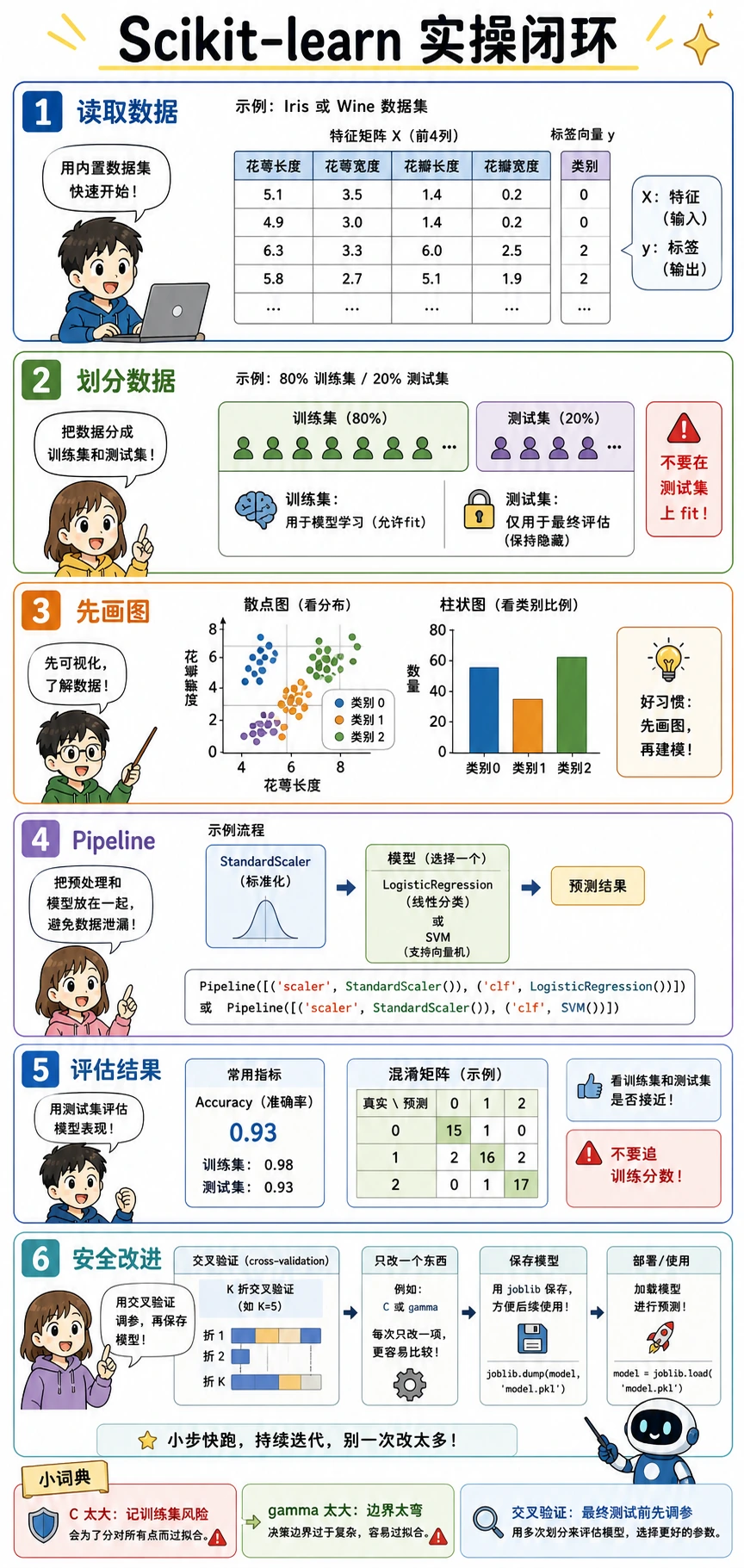
• 理解代码里的 X、y、X_train、X_test、y_train、y_test 分别是什么
• 用 Matplotlib 先看数据和结果，再相信模型分数
• 构建包含预处理和模型的 sklearn Pipeline
• 对比训练集和测试集分数，避免被过拟合骗到
• 用交叉验证一次只调一个关键设置
• 用 joblib 保存和重新加载训练好的 Pipeline

准备一个可运行单元

新建一个 Notebook 或 Python 文件，先运行下面的准备代码。

import numpy as np
import matplotlib.pyplot as plt

from sklearn.datasets import load_wine
from sklearn.model_selection import train_test_split, cross_val_score
from sklearn.pipeline import make_pipeline
from sklearn.preprocessing import StandardScaler
from sklearn.linear_model import LogisticRegression
from sklearn.metrics import ConfusionMatrixDisplay, classification_report

np.set_printoptions(precision=3, suppress=True)

如果 import sklearn 失败，在同一个 Python 环境里安装：

python -m pip install --upgrade scikit-learn matplotlib joblib

pip 用来安装包。python -m pip 的意思是“使用当前这个 Python 解释器对应的 pip”，可以避免安装到了一个环境、运行时却用了另一个环境的常见问题。

---

读取数据：分清特征和标签

在 sklearn 示例里，你会不断看到 X 和 y：

• X 是特征矩阵。每一行是一个样本，每一列是一个输入特征。
• y 是标签向量。每个值是模型要学习的答案。
• X.shape 表示 (样本数, 特征数)。
• y.shape 表示标签数量。

wine = load_wine()
X = wine.data
y = wine.target

print("X shape:", X.shape)
print("y shape:", y.shape)
print("Feature names:", wine.feature_names[:5], "...")
print("Class names:", wine.target_names.tolist())
print("First sample features:", np.round(X[0], 2))
print("First sample label:", y[0], "=>", wine.target_names[y[0]])

预期输出：

X shape: (178, 13)
y shape: (178,)
Feature names: ['alcohol', 'malic_acid', 'ash', 'alcalinity_of_ash', 'magnesium'] ...
Class names: ['class_0', 'class_1', 'class_2']
First sample features: [ 14.23   1.71   2.43  15.6  127.     2.8    3.06   0.28   2.29   5.64   1.04   3.92 1065.  ]
First sample label: 0 => class_0

新人检查点

训练任何模型之前，先回答三个问题：“一行代表什么？一列代表什么？标签是什么？”如果这三个问题还说不清，模型分数暂时也没太大意义。

---

Matplotlib 基础：先读懂图，再判断模型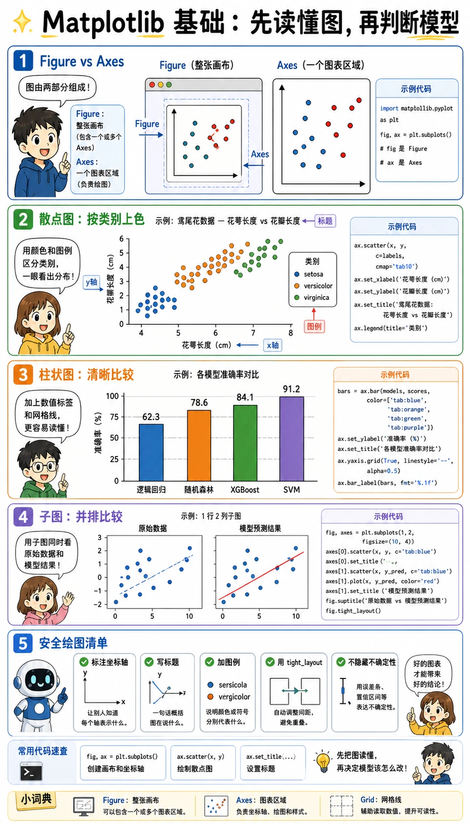

Matplotlib 有两个词很容易让新人混淆：

• Figure：整张画布。
• Axes：画布里的一个图表区域。

大多数入门代码可以照这个模板写：

fig, ax = plt.subplots(figsize=(6, 4))
ax.scatter(x_values, y_values)
ax.set_xlabel("x-axis label")
ax.set_ylabel("y-axis label")
ax.set_title("Chart title")
ax.grid(True, alpha=0.3)
plt.tight_layout()
plt.show()

现在画出 Wine 数据集的两个特征：

feature_x = 0  # alcohol
feature_y = 6  # flavanoids

fig, ax = plt.subplots(figsize=(7, 5))
scatter = ax.scatter(
    X[:, feature_x],
    X[:, feature_y],
    c=y,
    cmap="viridis",
    s=45,
    alpha=0.85,
)

ax.set_xlabel(wine.feature_names[feature_x])
ax.set_ylabel(wine.feature_names[feature_y])
ax.set_title("Wine data: two-feature view")
ax.grid(True, alpha=0.3)
ax.legend(
    handles=scatter.legend_elements()[0],
    labels=wine.target_names.tolist(),
    title="Class",
)

plt.tight_layout()
plt.show()

观察时重点看：

• 类别之间是否已经有一点分开？
• 是否有明显重叠区域？
• 有没有某个特征的数值范围特别大？

这就是可视化的价值：它让你先感受问题难不难，再看模型分数。

---

划分数据：让测试集保持隐藏

train_test_split 会创建训练集和测试集。

• 训练集：允许模型学习。
• 测试集：只用于最后评估。
• stratify=y：让训练集和测试集里的类别比例尽量一致。
• random_state：让划分结果可复现。

X_train, X_test, y_train, y_test = train_test_split(
    X,
    y,
    test_size=0.2,
    random_state=42,
    stratify=y,
)

print("X_train:", X_train.shape, "y_train:", y_train.shape)
print("X_test: ", X_test.shape, "y_test: ", y_test.shape)

预期输出：

X_train: (142, 13) y_train: (142,)
X_test:  (36, 13) y_test:  (36,)

最常见的新手错误

不要在测试集上运行 fit。测试集是最后考试。如果预处理或调参从测试集学习了信息，报告出来的分数就会偏乐观。

---

构建 Pipeline：预处理加模型

逻辑回归、SVM、KNN 等模型都比较依赖特征尺度。Wine 数据集的列单位差异很大，所以我们把 StandardScaler 放在模型前面。

model = make_pipeline(
    StandardScaler(),
    LogisticRegression(max_iter=1000, random_state=42),
)

model.fit(X_train, y_train)

train_score = model.score(X_train, y_train)
test_score = model.score(X_test, y_test)

print(f"训练准确率：{train_score:.1%}")
print(f"测试准确率：{test_score:.1%}")

预期输出：

训练准确率：100.0%
测试准确率：100.0%

Pipeline 的价值在于保持正确顺序：

1. 对训练数据：StandardScaler.fit_transform，然后模型 fit
2. 对测试数据：StandardScaler.transform，然后模型 predict

这个细节可以防止数据泄漏。

---

预测并查看具体样本

分数有用，但新人也应该看几个具体预测。

y_pred = model.predict(X_test)
proba = model.predict_proba(X_test[:5])

for i in range(5):
    predicted_name = wine.target_names[y_pred[i]]
    true_name = wine.target_names[y_test[i]]
    confidence = proba[i].max()
    print(f"Sample {i}: predicted={predicted_name}, true={true_name}, confidence={confidence:.1%}")

示例输出：

Sample 0: predicted=class_0, true=class_0, confidence=99.9%
Sample 1: predicted=class_1, true=class_1, confidence=99.9%
Sample 2: predicted=class_0, true=class_0, confidence=99.5%
Sample 3: predicted=class_1, true=class_1, confidence=99.7%
Sample 4: predicted=class_2, true=class_2, confidence=99.9%

predict 返回最终类别。predict_proba 返回每个类别的概率分布。概率在需要阈值、人工复核、风险排序时很有用。

---

用混淆矩阵和报告评估

准确率会隐藏“到底哪些类别混了”。混淆矩阵会把真实标签和预测标签放在两个轴上。

fig, ax = plt.subplots(figsize=(5, 5))
ConfusionMatrixDisplay.from_estimator(
    model,
    X_test,
    y_test,
    display_labels=wine.target_names,
    cmap="Blues",
    ax=ax,
    colorbar=False,
)
ax.set_title("Confusion matrix on test set")
plt.tight_layout()
plt.show()

print(classification_report(y_test, y_pred, target_names=wine.target_names))

阅读方式：

• 对角线是预测正确。
• 非对角线是预测错误。
• Precision 问：“预测成 A 的样本里，有多少真的是 A？”
• Recall 问：“真实是 A 的样本里，我们抓住了多少？”
• F1 会综合 precision 和 recall。

---

用同一套流程比较多个模型

因为 sklearn 有统一 API，模型对比会很方便。

from sklearn.tree import DecisionTreeClassifier
from sklearn.neighbors import KNeighborsClassifier
from sklearn.svm import SVC

models = {
    "Logistic Regression": make_pipeline(
        StandardScaler(),
        LogisticRegression(max_iter=1000, random_state=42),
    ),
    "Decision Tree": DecisionTreeClassifier(max_depth=4, random_state=42),
    "KNN": make_pipeline(StandardScaler(), KNeighborsClassifier(n_neighbors=5)),
    "SVM": make_pipeline(StandardScaler(), SVC(kernel="rbf", C=1.0, gamma="scale")),
}

results = {}
for name, clf in models.items():
    clf.fit(X_train, y_train)
    results[name] = {
        "train": clf.score(X_train, y_train),
        "test": clf.score(X_test, y_test),
    }
    print(f"{name:20s} train={results[name]['train']:.1%} test={results[name]['test']:.1%}")

示例输出：

Logistic Regression  train=100.0% test=100.0%
Decision Tree        train=99.3% test=94.4%
KNN                  train=97.9% test=97.2%
SVM                  train=100.0% test=100.0%

把对比画出来：

fig, ax = plt.subplots(figsize=(9, 5))
names = list(results.keys())
x = np.arange(len(names))
width = 0.35

train_scores = [results[name]["train"] for name in names]
test_scores = [results[name]["test"] for name in names]

bars_train = ax.bar(x - width / 2, train_scores, width, label="Train", color="steelblue")
bars_test = ax.bar(x + width / 2, test_scores, width, label="Test", color="coral")

ax.set_xticks(x)
ax.set_xticklabels(names, rotation=15, ha="right")
ax.set_ylabel("Accuracy")
ax.set_title("Model comparison on Wine dataset")
ax.set_ylim(0.8, 1.05)
ax.legend()
ax.grid(axis="y", alpha=0.3)
ax.bar_label(bars_train, fmt="%.2f", padding=3)
ax.bar_label(bars_test, fmt="%.2f", padding=3)

plt.tight_layout()
plt.show()

如果训练分数远高于测试分数，要警惕过拟合。如果两个分数都低，可能是欠拟合、特征弱或模型不适合。

---

用交叉验证安全调参

不要直接在测试集上调超参数。应该在训练集内部做交叉验证。

candidates = [0.01, 0.1, 1.0, 10.0, 100.0]

for C in candidates:
    clf = make_pipeline(
        StandardScaler(),
        LogisticRegression(C=C, max_iter=1000, random_state=42),
    )
    scores = cross_val_score(clf, X_train, y_train, cv=5, scoring="accuracy")
    print(f"C={C:<6} CV accuracy={scores.mean():.1%} ± {scores.std():.1%}")

示例输出：

C=0.01   CV accuracy=95.8% ± 3.1%
C=0.1    CV accuracy=98.6% ± 1.8%
C=1.0    CV accuracy=98.6% ± 1.8%
C=10.0   CV accuracy=97.9% ± 2.6%
C=100.0  CV accuracy=97.9% ± 2.6%

比具体结果更重要的是习惯：

1. 先切出测试集，并且不要碰它。
2. 在训练集上用交叉验证调参。
3. 选出最好的设置。
4. 用全部训练数据训练最终模型。
5. 最后只在测试集上评估一次。

---

保存并重新加载最终 Pipeline

import joblib

final_model = make_pipeline(
    StandardScaler(),
    LogisticRegression(C=1.0, max_iter=1000, random_state=42),
)
final_model.fit(X_train, y_train)

joblib.dump(final_model, "wine_classifier.joblib")
loaded_model = joblib.load("wine_classifier.joblib")

same_predictions = np.array_equal(
    final_model.predict(X_test),
    loaded_model.predict(X_test),
)

print("Loaded model test accuracy:", f"{loaded_model.score(X_test, y_test):.1%}")
print("Predictions are identical:", same_predictions)

预期输出：

Loaded model test accuracy: 100.0%
Predictions are identical: True

安全提醒

只加载你信任的 joblib 或 pickle 文件。加载序列化的 Python 对象可能执行代码。

---

留下的证据

学完这一页，至少保留这张证据卡：

机器学习问题

监督学习、无监督学习、评估或特征工程任务

基线

最简单的 sklearn/建模循环和固定的训练/测试划分

输出

预测、指标、图表，或模型决策备注

失败检查

数据泄漏、目标不清、基线薄弱或指标不匹配

期望产出

带指标和一个失败观察的最小 ML 循环

常见错误与快速修复

错误 / 现象	可能原因	修复方式
NameError: name 'X_train' is not defined	跳过了数据划分单元	先运行数据读取和 train_test_split 单元
ValueError: Found input variables with inconsistent numbers of samples	X 和 y 长度不一致	划分前打印 X.shape 和 y.shape
训练分数很高，测试分数低很多	过拟合	降低模型复杂度、用交叉验证、增加数据或改善特征
Notebook 分数很好，真实使用很差	数据泄漏或预处理不一致	保存和使用完整 Pipeline，不要只保存模型
图表标签重叠	图太小或布局没调整	增大 figsize，旋转标签，使用 plt.tight_layout()

跟练任务

用 load_iris() 重复完整流程：

1. 打印 X.shape、y.shape、特征名和类别名。
2. 用两个特征画散点图。
3. 用 train_test_split(..., stratify=y) 划分数据。
4. 训练 Pipeline(StandardScaler(), LogisticRegression(...))。
5. 打印训练和测试准确率。
6. 画混淆矩阵。
7. 用交叉验证调 C。
8. 用 joblib 保存并重新加载模型。

操作参考与检查点

1. load_iris() 应该得到 150 行、4 个数值特征和 3 个类别名。如果 X.shape[0] 和 y.shape[0] 不一致，说明特征/标签拆分错了。
2. 散点图应该让你看到，有些特征组合更能分开类别。它是结构检查，不是模型已经足够好的证明。
3. stratify=y 可以让训练集和测试集的类别比例更稳定，即使 Iris 比较均衡，也建议保留这个习惯。
4. Pipeline 应该同时包含 StandardScaler() 和 LogisticRegression(...)，这样标准化只会从训练数据学习参数。
5. 训练和测试准确率应该接近。如果训练明显高、测试低，就要检查过拟合或划分不稳定。
6. 混淆矩阵告诉你哪些类别容易互相混淆。先看它，再决定是否换模型或改特征。
7. C 应该在训练侧用交叉验证选择，最后只检查一次测试集。不要反复看测试分数来挑 C。
8. joblib 重新加载后，预测结果应该和原模型一致。只加载你信任的序列化文件。

这节最该带走什么

如果第五章有一个实操闭环，就是这句话：

先看数据，再划分数据；划分后再 fit；用 Pipeline 串起预处理和模型；用隐藏数据评估；用交叉验证改进；保存完整工作流。