6.2.3 PyTorch 基础

本节定位

这页不是 API 目录。目标是建立每次写 PyTorch 模型前都要有的反射：训练前先读 shape、dtype、device 和运算含义。

学习目标

• 从 Python 和 NumPy 数据创建张量。
• 读懂 shape、dtype、device 和每一维的含义。
• 区分逐元素运算和矩阵乘法。
• 有意识地使用 broadcasting，而不是让它悄悄发生。
• 跑通一个小型前向过程，得到 logits、概率、预测和 loss。

---

先看 Tensor 生命周期

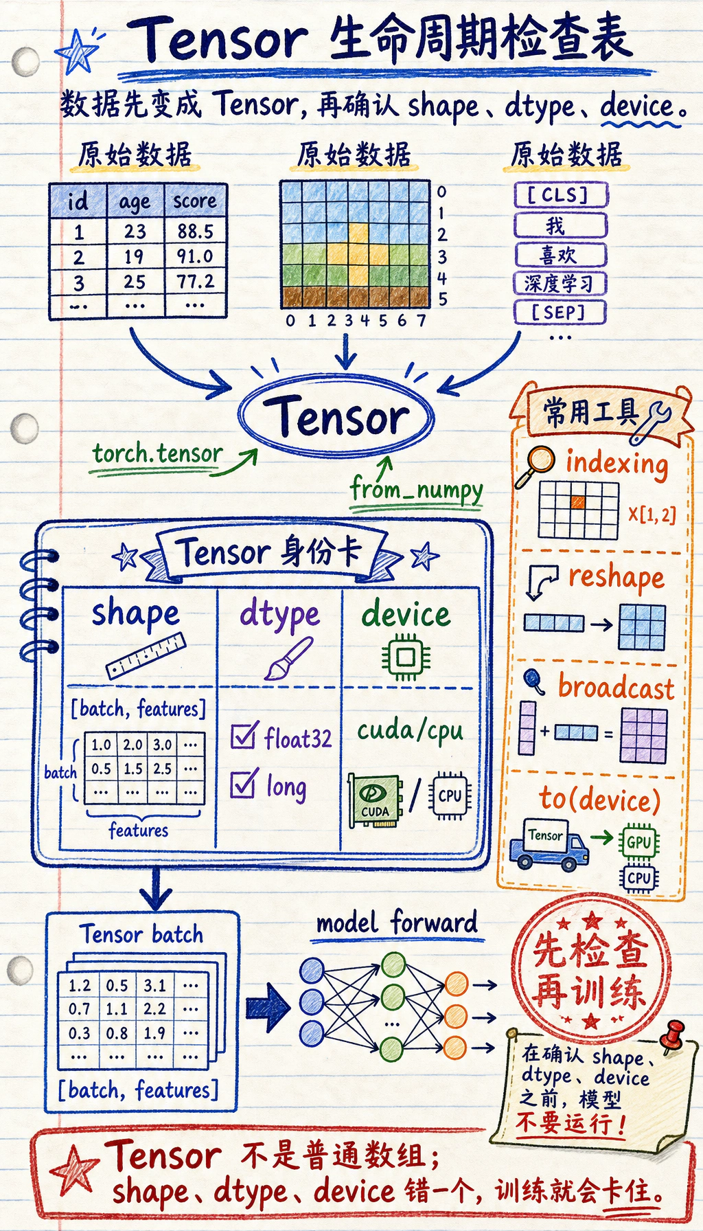
大多数 PyTorch 数据会走这条路径：

原始数据→tensor→shape/dtype/device 检查→运算/模型→loss→梯度/更新

新手最容易犯的错是直接跳到模型。更稳的习惯是：数据进模型前先检查张量。

Tensor 是带训练信息的数据

最短的实用定义是：

张量是 PyTorch 能计算、能跨设备移动、必要时还能追踪梯度的多维数组。

和 NumPy 数组相比，PyTorch 张量多了两个深度学习能力：

• device：张量可以放在 CPU、GPU 或 Apple MPS 上。
• requires_grad：张量可以参与自动求导。

常见 shape：

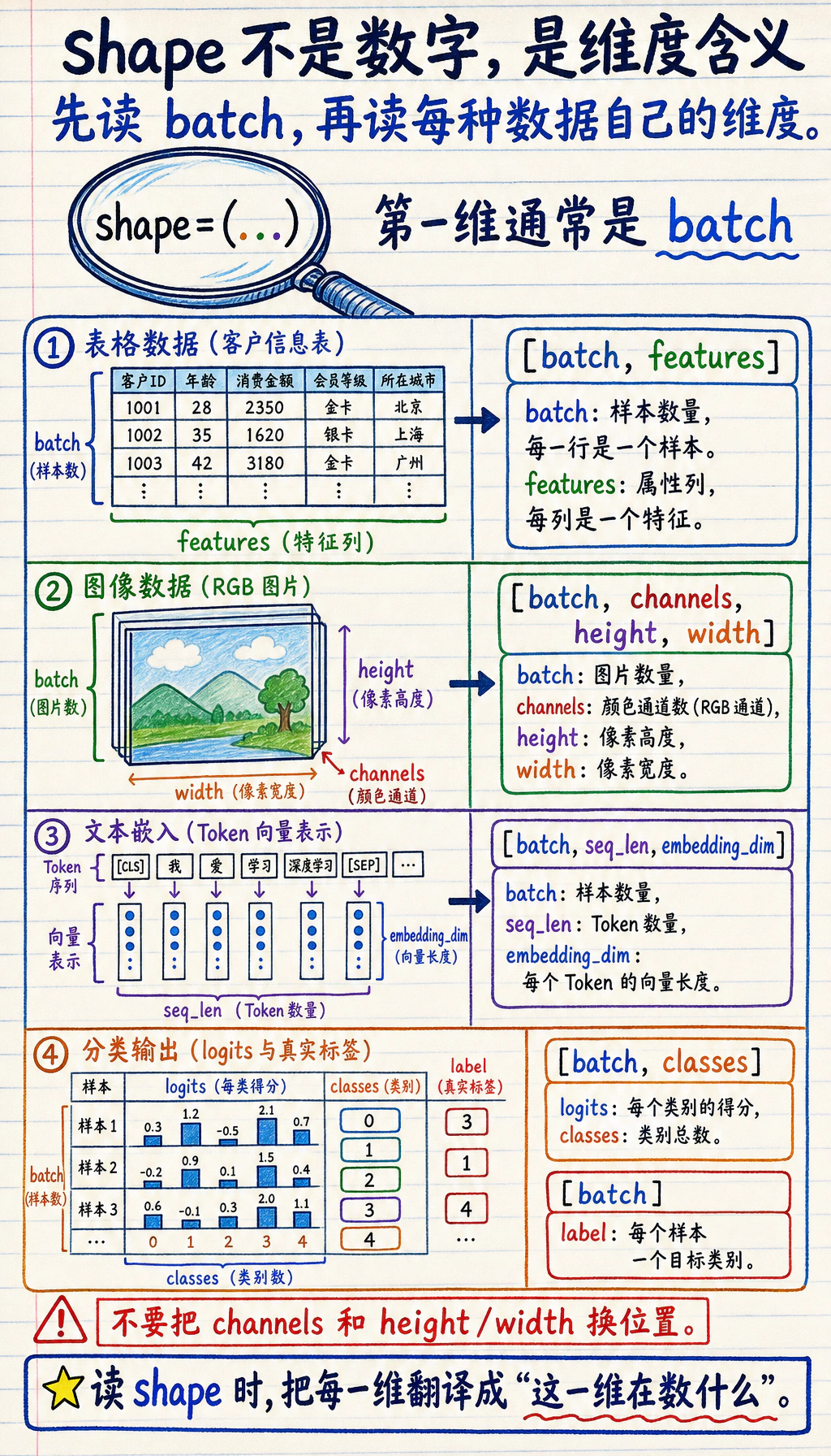
数据	常见 shape	含义
表格 batch	[batch, features]	行是样本，列是特征
分类标签	[batch]	每个样本一个整数类别 id
图片 batch	[batch, channels, height, width]	PyTorch 图片惯例
文本向量	[batch, seq_len, embedding_dim]	token 对应的向量表示
logits	[batch, classes]	softmax 前的原始类别分数

实验 1：做数学运算前先检查张量

先运行这段。它会帮你建立后面每个训练循环都要用的检查习惯。

import torch


def describe(name, tensor, meaning):
    print(
        f"{name}: shape={tuple(tensor.shape)} "
        f"dtype={tensor.dtype} "
        f"device={tensor.device} "
        f"meaning={meaning}"
    )


X = torch.tensor(
    [
        [1.0, 2.0, 3.0],
        [4.0, 5.0, 6.0],
    ]
)
y = torch.tensor([0, 1], dtype=torch.long)

describe("X", X, "[batch, features]")
describe("y", y, "[batch]")

print("ndim:", X.ndim)
print("numel:", X.numel())
print("first row:", X[0])
print("feature means:", X.mean(dim=0))

预期输出：

X: shape=(2, 3) dtype=torch.float32 device=cpu meaning=[batch, features]
y: shape=(2,) dtype=torch.int64 device=cpu meaning=[batch]
ndim: 2
numel: 6
first row: tensor([1., 2., 3.])
feature means: tensor([2.5000, 3.5000, 4.5000])

重点看：

• X 是 float32，这通常是模型输入类型。
• y 是 int64，也就是 torch.long，这是 CrossEntropyLoss 对分类标签的要求。
• dim=0 会沿 batch 方向聚合，得到每个特征的均值。

实验 2：从特征到 logits

现在手写一个非常小的分类前向过程。它模拟的是 nn.Linear 内部做的事情。

import torch
import torch.nn as nn


def describe(name, tensor, meaning):
    print(
        f"{name}: shape={tuple(tensor.shape)} "
        f"dtype={tensor.dtype} "
        f"device={tensor.device} "
        f"meaning={meaning}"
    )


X = torch.tensor(
    [
        [1.0, 2.0, 3.0],
        [4.0, 5.0, 6.0],
    ]
)
y = torch.tensor([0, 1], dtype=torch.long)

W = torch.tensor(
    [
        [0.1, 0.2],
        [0.3, -0.1],
        [0.5, 0.4],
    ]
)
b = torch.tensor([0.01, -0.02])

logits = X @ W + b
probs = torch.softmax(logits, dim=1)
pred = probs.argmax(dim=1)
loss = nn.CrossEntropyLoss()(logits, y)

describe("logits", logits, "[batch, classes]")
print("logits:", torch.round(logits * 100) / 100)
print("probabilities:", torch.round(probs * 1000) / 1000)
print("prediction:", pred)
print("loss:", round(loss.item(), 3))

预期输出：

logits: shape=(2, 2) dtype=torch.float32 device=cpu meaning=[batch, classes]
logits: tensor([[2.2100, 1.1800],
        [4.9100, 2.6800]])
probabilities: tensor([[0.7370, 0.2630],
        [0.9030, 0.0970]])
prediction: tensor([0, 0])
loss: 1.319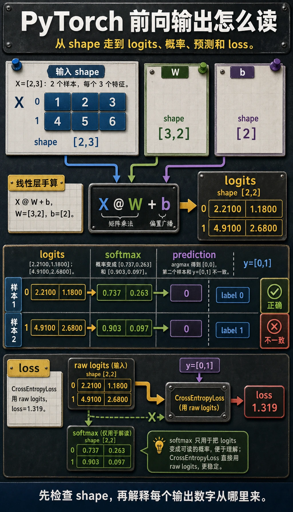

仔细读 shape：

• X 是 [2, 3]：两个样本、三个特征。
• W 是 [3, 2]：三个输入特征、两个输出类别。
• X @ W 变成 [2, 2]：每个样本一组类别分数。
• b 是 [2]，会被广播到整个 batch。
• CrossEntropyLoss 接收原始 logits，不是 softmax 后的概率。

重要

PyTorch 多分类时，把原始 logits 传给 nn.CrossEntropyLoss()。不要在 loss 前手动做 softmax。softmax 只用于检查概率或做预测解释。

真正常用的 shape 操作

用 reshape、unsqueeze 和 squeeze 把 shape 调成下一步运算需要的样子。

import torch

x = torch.arange(12)
grid = x.reshape(3, 4)
batch = grid.unsqueeze(0)
restored = batch.squeeze(0)

print("x:", tuple(x.shape))
print("grid:", tuple(grid.shape))
print("batch:", tuple(batch.shape))
print("restored:", tuple(restored.shape))

预期输出：

x: (12,)
grid: (3, 4)
batch: (1, 3, 4)
restored: (3, 4)

实际含义：

• reshape(3, 4)：把同样的 12 个元素重新组织成表。
• unsqueeze(0)：增加一个 batch 维度。
• squeeze(0)：去掉大小为 1 的 batch 维度。

除非你明确知道为什么要用 view，否则先用 reshape。当内存布局不是连续时，reshape 更宽容。

Broadcasting：好用，但要检查方向

Broadcasting 的意思是：当 shape 兼容时，PyTorch 会把小张量自动扩展成大张量的形状。

import torch

X = torch.tensor(
    [
        [1.0, 2.0, 3.0],
        [4.0, 5.0, 6.0],
    ]
)

feature_mean = X.mean(dim=0)
centered = X - feature_mean

print("feature_mean:", feature_mean)
print("centered:", centered)

预期输出：

feature_mean: tensor([2.5000, 3.5000, 4.5000])
centered: tensor([[-1.5000, -1.5000, -1.5000],
        [ 1.5000,  1.5000,  1.5000]])

这里 feature_mean 的 shape 是 [3]，X 的 shape 是 [2, 3]。PyTorch 会把同一组特征均值从每一行里减掉。

依赖 broadcasting 前，把 shape 写在代码旁边：

# X: [batch, features]
# feature_mean: [features]
centered = X - feature_mean

这条小注释能避免很多静默逻辑错误。

Device 和 NumPy 转换

真实训练代码必须让张量待在同一个 device 上。这个写法可以兼容 CPU、CUDA 和 Apple Silicon MPS。

import torch

if torch.cuda.is_available():
    device = torch.device("cuda")
elif torch.backends.mps.is_available():
    device = torch.device("mps")
else:
    device = torch.device("cpu")

X = torch.tensor([[1.0, 2.0, 3.0]])
X = X.to(device)

print("device:", X.device)

如果要转回 NumPy 画图或分析，先 detach，再搬回 CPU：

arr = X.detach().cpu().numpy()
print(type(arr), arr.shape)

为什么顺序重要：

• .detach() 离开梯度图。
• .cpu() 确保 NumPy 能读到数据。
• .numpy() 转成 NumPy 数组。

常见错误模式

现象	可能原因	修复方式
mat1 and mat2 shapes cannot be multiplied	矩阵乘法维度不对	在 @ 或 nn.Linear 前打印两个 shape
expected scalar type Long	分类 loss 的标签是 float	使用 y = y.long()
Expected all tensors to be on the same device	模型和数据不在同一设备	用 .to(device) 移动模型和数据
loss 能跑但结果怪	broadcasting 方向不是你以为的方向	写出两个 shape 并确认扩展方式
NumPy 转换失败	张量在 GPU 上或还连着梯度图	用 tensor.detach().cpu().numpy()

快速排错清单

张量进模型前，先打印：

print("shape:", tuple(X.shape))
print("dtype:", X.dtype)
print("device:", X.device)
print("meaning: [batch, features]")

进 loss 前，检查：

print("logits:", tuple(logits.shape), logits.dtype)
print("labels:", tuple(y.shape), y.dtype)

多分类里最常见的组合是：

logits: [batch, classes], float32
labels: [batch], int64 / long

留下的证据

继续前，保存一条小的 tensor 检查笔记：

输入形状

[batch, features]

logits 形状

[batch, classes]

标签形状

[batch]

标签数据类型

CrossEntropyLoss 使用 torch.long

设备检查

模型和数据在同一设备上

这是后面调试 PyTorch 代码最快的方法。大多数早期错误都是 shape、dtype、device 或 broadcasting 错误，只是被长长的报错堆栈藏起来了。

练习

1. 把实验 2 里的 X 从两个样本改成三个样本。哪些 shape 会变，哪些不会变？
2. 创建 shape 为 [batch, 1] 的标签，再用 squeeze(1) 修成 CrossEntropyLoss 能接受的形状。
3. 把 X、W 和 b 移到 device。如果只移动其中一个，会得到什么错误？
4. 把 X @ W 改成 X * W。为什么它会失败，或者表达完全不同的含义？

参考实现与讲解

1. batch 维度会从 2 变成 3。feature 数、class 数和参数 shape 不变，除非你也改了输入特征数或输出类别数。
2. CrossEntropyLoss 需要形状类似 [batch] 的类别标签，并且通常是 torch.long。squeeze(1) 会去掉多余的单例维度，让 loss 看到每个样本一个类别 id。
3. 会出现 device mismatch 一类错误，例如有些 tensor 在 CPU，有些在 GPU。PyTorch 中参与同一个运算的模型参数和输入 tensor 必须在同一个 device 上。
4. @ 是矩阵乘法，会得到 class logits；* 是逐元素乘法，shape 不匹配时会报错，shape 能广播时也表达了完全不同的运算。

小结

• PyTorch 基础不是背很多函数，而是匹配 shape、dtype、device 和运算含义。
• @ 是矩阵乘法；* 是逐元素乘法。
• CrossEntropyLoss 需要原始 logits 和 long 标签。
• Broadcasting 很强，但你必须知道哪一维在被扩展。