6.3.3 CNN 基本结构

本节定位

上一页解释了一个 kernel 如何扫描一个局部窗口。本页把这些部件组装成完整 CNN，并逐层追踪 shape，让模型不再只是图上的几个方块。

学习目标

• 描述 image -> conv block -> feature map -> classifier head -> logits 的路径。
• 解释为什么通道数通常增加，而高宽通常减小。
• 运行一个小卷积块，并读懂输出 shape。
• 用 PyTorch 搭建完整的 TinyCNN。
• 从工程角度比较 Flatten 和 Global Average Pooling（GAP）。

---

先看整体流水线

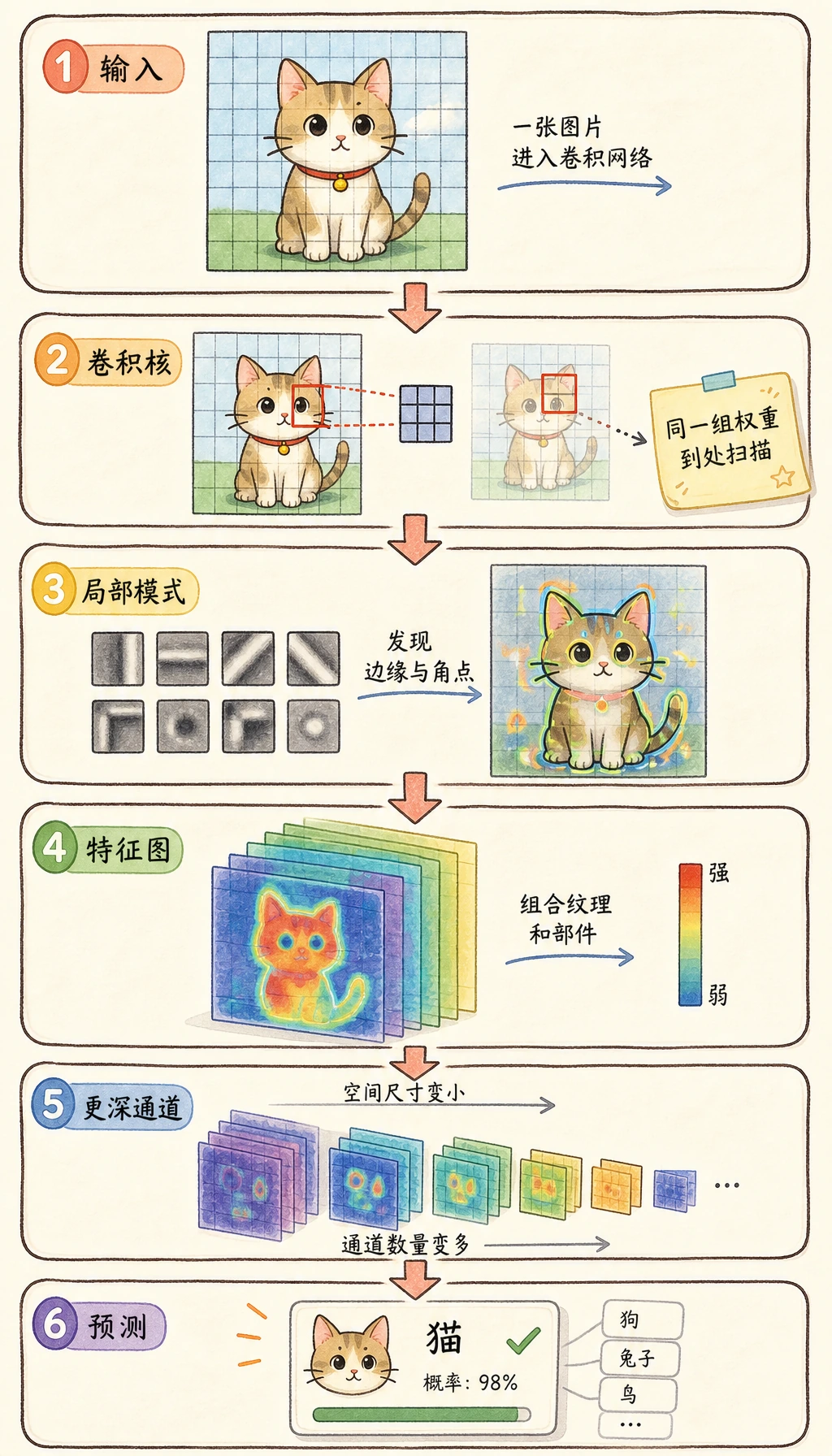
按从左到右读图：

图像→低层特征→压缩后的 feature map→分类头→类别分数

CNN 通常分成两部分：

部分	作用	常见层
feature extractor	把像素变成有用的 feature map	Conv2d、ReLU、BatchNorm2d、MaxPool2d
classifier head	把最后的 feature map 变成类别分数	Flatten 或 GAP、Linear

最后一层输出通常叫 logits：也就是进入 softmax 之前的原始类别分数。

通道数变多，空间尺寸变小

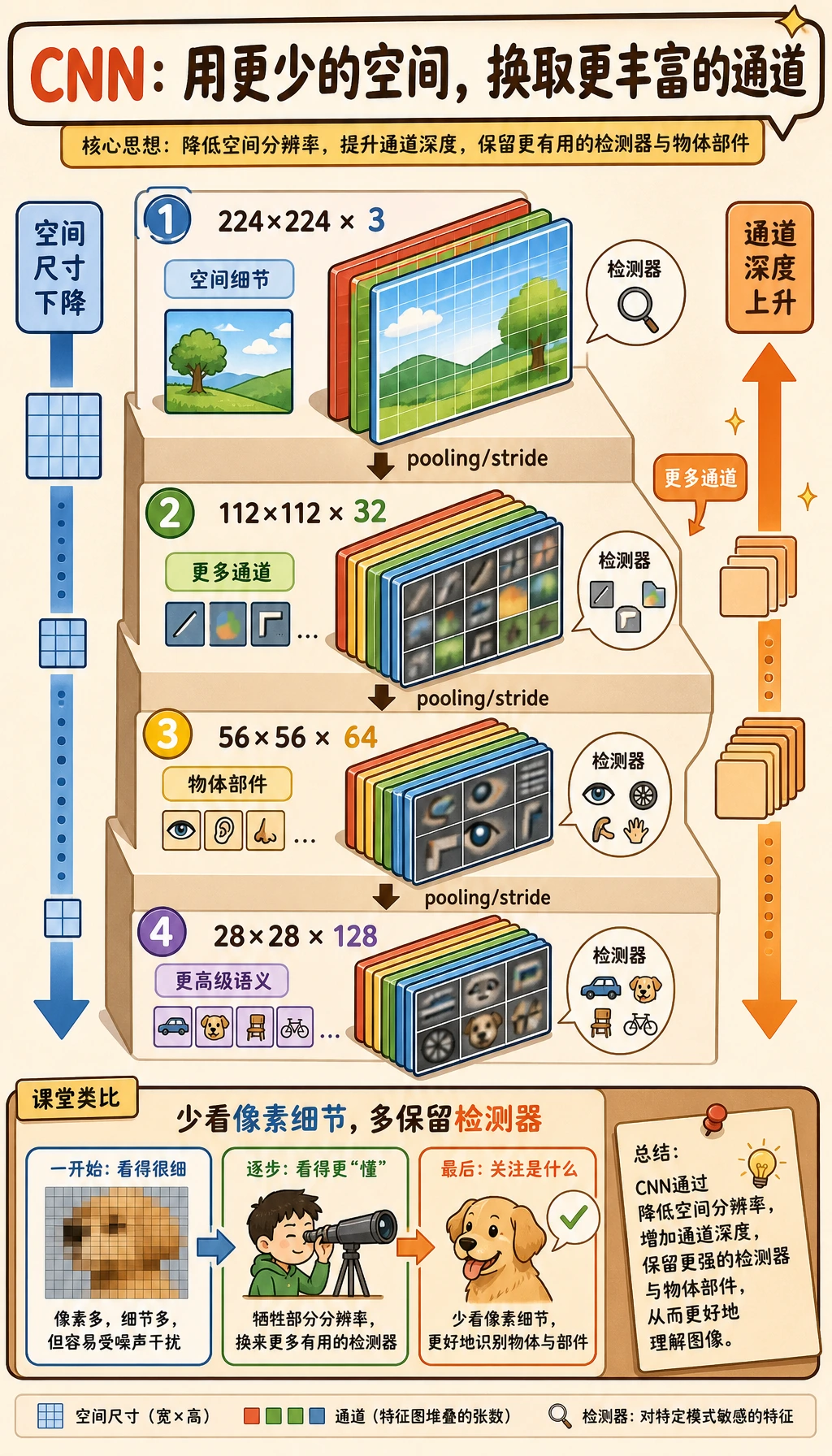
浅层保留更多空间细节。深层保留更少像素位置，但保存更多特征类型。

阶段	shape 直觉	含义
input	[N, 3, 32, 32]	RGB 图像
early feature	[N, 16, 32, 32]	多种边缘、纹理检测器
after pooling	[N, 16, 16, 16]	更小的图，保留局部最强信号
deeper feature	[N, 64, 8, 8]	更抽象的模式

这是 CNN 设计的核心取舍：

• 更少的空间位置可以减少计算；
• 更多的通道可以存储更丰富的视觉证据；
• 分类头应该看到足够语义，而不是每一个原始像素。

实验 1：手算 MaxPool

MaxPool2d(2) 会在每个 2 x 2 窗口里保留最大值。

import numpy as np

feature_map = np.array(
    [
        [1, 3, 2, 0],
        [4, 6, 1, 2],
        [0, 1, 5, 3],
        [2, 4, 1, 7],
    ],
    dtype=np.float32,
)

pooled = np.array(
    [
        [feature_map[0:2, 0:2].max(), feature_map[0:2, 2:4].max()],
        [feature_map[2:4, 0:2].max(), feature_map[2:4, 2:4].max()],
    ]
)

print("maxpool_lab")
print(pooled)

预期输出：

maxpool_lab
[[6. 2.]
 [4. 7.]]

池化会丢掉一部分细节，但它保留了局部最强响应。对分类任务来说，这通常是有用的偏置：模型更关心某个特征是否出现，而不是它精确出现在哪个像素。

实验 2：运行一个卷积块

一个基础 CNN block 是：

Conv2d→activation→optional pooling

运行：

import torch
from torch import nn

block = nn.Sequential(
    nn.Conv2d(3, 8, kernel_size=3, padding=1),
    nn.ReLU(),
    nn.MaxPool2d(kernel_size=2),
)

x = torch.randn(2, 3, 32, 32)
y = block(x)

print("block_lab")
print("input:", tuple(x.shape))
print("output:", tuple(y.shape))

预期输出：

block_lab
input: (2, 3, 32, 32)
output: (2, 8, 16, 16)

变化在哪里：

• batch 仍然是 2；
• 通道从 3 变成 8；
• 高和宽因为 MaxPool2d(2) 从 32 缩到 16。

实际项目里常见的变体是：

Conv2d→BatchNorm2d→ReLU

BatchNorm2d 可以在训练时稳定 feature 的尺度。它很有用，但第一次搭模型时，先把 shape 流程看清楚更重要。

实验 3：搭建完整 Tiny CNN

这个模型接收灰度 28 x 28 图像，并输出 10 个类别分数。

import torch
from torch import nn


class TinyCNN(nn.Module):
    def __init__(self, num_classes=10):
        super().__init__()
        self.conv1 = nn.Conv2d(1, 8, kernel_size=3, padding=1)
        self.pool1 = nn.MaxPool2d(2)
        self.conv2 = nn.Conv2d(8, 16, kernel_size=3, padding=1)
        self.pool2 = nn.MaxPool2d(2)
        self.classifier = nn.Sequential(
            nn.Flatten(),
            nn.Linear(16 * 7 * 7, 64),
            nn.ReLU(),
            nn.Linear(64, num_classes),
        )

    def forward(self, x):
        print("shape_trace")
        print(f"{'input':<8} {tuple(x.shape)}")
        x = torch.relu(self.conv1(x))
        print(f"{'conv1':<8} {tuple(x.shape)}")
        x = self.pool1(x)
        print(f"{'pool1':<8} {tuple(x.shape)}")
        x = torch.relu(self.conv2(x))
        print(f"{'conv2':<8} {tuple(x.shape)}")
        x = self.pool2(x)
        print(f"{'pool2':<8} {tuple(x.shape)}")
        x = self.classifier(x)
        print(f"{'logits':<8} {tuple(x.shape)}")
        return x


model = TinyCNN(num_classes=10)
x = torch.randn(4, 1, 28, 28)
_ = model(x)

预期输出：

shape_trace
input    (4, 1, 28, 28)
conv1    (4, 8, 28, 28)
pool1    (4, 8, 14, 14)
conv2    (4, 16, 14, 14)
pool2    (4, 16, 7, 7)
logits   (4, 10)

最后 shape 是 [4, 10]，因为 batch 里有 4 张图，每张图输出 10 个分数。

像工程师一样读结构

看 CNN 时，不要只读层名，要追踪每个边界的 tensor contract。

代码行	要检查的约定
Conv2d(1, 8, ...)	输入必须有 1 个通道
MaxPool2d(2)	高和宽会除以 2
Conv2d(8, 16, ...)	上一层输出通道必须是 8
Linear(16 * 7 * 7, 64)	flatten 后的特征数必须和真实 feature map 一致
最后的 Linear(..., 10)	输出维度必须等于类别数

大多数 CNN 报错都是 contract 报错：到达某一层的 tensor shape 和这层期待的不一样。

Flatten 和 Global Average Pooling

Flatten 会把所有空间位置拉成一个长向量：

[N, 16, 7, 7] -> [N, 784]

GAP 每个通道只保留一个平均值：

[N, 16, 7, 7] -> [N, 16]

比较参数量：

from torch import nn


def count_params(module):
    return sum(p.numel() for p in module.parameters() if p.requires_grad)


flatten_head = nn.Linear(16 * 7 * 7, 10)
gap_head = nn.Linear(16, 10)

print("head_param_lab")
print("flatten head:", count_params(flatten_head))
print("gap head    :", count_params(gap_head))

预期输出：

head_param_lab
flatten head: 7850
gap head    : 170

取舍可以这样看：

Head	优点	代价
Flatten + Linear	简单，能使用位置相关细节	参数多，输入尺寸更固定
GAP + Linear	紧凑，更容易适配变化的空间尺寸	可能丢掉精细位置信息

现代 CNN 分类器经常用 GAP，因为它能降低过拟合风险，并让 head 更小。

留下的证据

保留一条 CNN shape trace：

输入

[batch, channels, height, width]

卷积后状态

通道变化，空间尺寸随 padding/stride 变化

池化后

高和宽缩小

前一层头部

已知展平后的大小或 GAP 输出

logits 形状

[batch, num_classes]

头部选择

Flatten 适合位置相关细节，GAP 适合紧凑分类器

常见错误

错误	现象	修复
通道顺序写错	expected input ... to have C channels	PyTorch 中使用 [N, C, H, W]
Linear 输入尺寸写错	矩阵乘法 shape 报错	在 Flatten 前打印 shape
太早、太多 pooling	feature map 变得过小	每个 block 后追踪 H 和 W
把 logits 当概率	loss 或评估理解混乱	CrossEntropyLoss 直接吃 logits；展示时再 softmax
加了 BatchNorm 却不理解模式	train/eval 行为不同	训练用 model.train()，评估用 model.eval()

练习

1. 把 conv2 的输出通道从 16 改成 32，哪些行必须跟着改？
2. 用 AdaptiveAvgPool2d((1, 1))、Flatten 和 Linear(16, 10) 替换分类头。
3. 删除一个 pooling 层，先预测新的 flatten 尺寸，再运行代码验证。
4. 在 conv1 后加入 BatchNorm2d(8)，确认 shape 不变。
5. 针对 RGB 64 x 64 输入，手写每一层后的 shape。

参考实现与讲解

1. conv2 输出变成 32 个通道后，后面的分类头输入维度必须同步修改；如果还有下一层卷积，它的 in_channels 也要改。
2. GAP 分类头会把空间尺寸压成 1 x 1，所以 Linear 只依赖通道数，结构更不容易被输入尺寸卡住。
3. 删除 pooling 会让特征图空间尺寸更大，Flatten 后的特征数也随之增加。先算 shape 再改 Linear。
4. BatchNorm2d(8) 对每个通道做归一化，不改变 batch、channel、height、width 的形状。
5. 形状追踪应按 conv/pool/conv/pool/head 顺序写清楚。最重要的是确认 channel 变化和空间尺寸变化分别发生在哪一层。

小结

• CNN 是 feature extractor 加 classifier head。
• 卷积块增加特征通道；pooling 或 stride 通常降低空间尺寸。
• shape tracing 是调试 CNN 结构最快的方法。
• Flatten 简单但参数多；GAP 更紧凑，在现代 CNN 中很常见。
• 好的 CNN 设计重点是控制信息流，而不是盲目堆层数。