6.5.2 注意力机制

本节定位

RNN 是一步步传信息。注意力让一个 token 直接看其他 token，并判断哪些更重要。这是 Transformer 背后的核心转变。

学习目标

• 解释为什么注意力有助于长距离依赖。
• 通过检索类比理解 Query、Key、Value。
• 手算 scaled dot-product attention。
• 使用 causal mask 防止偷看未来。
• 读懂 PyTorch 中 nn.MultiheadAttention 的 shape。

---

先看 Q/K/V

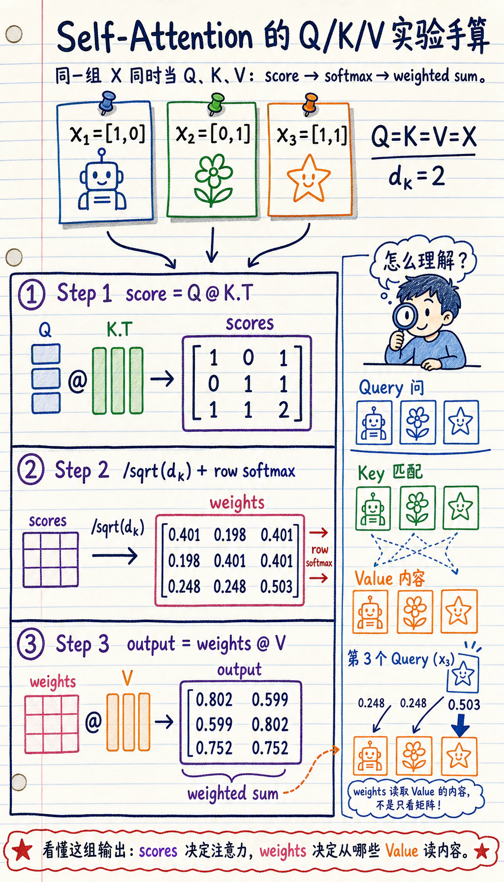
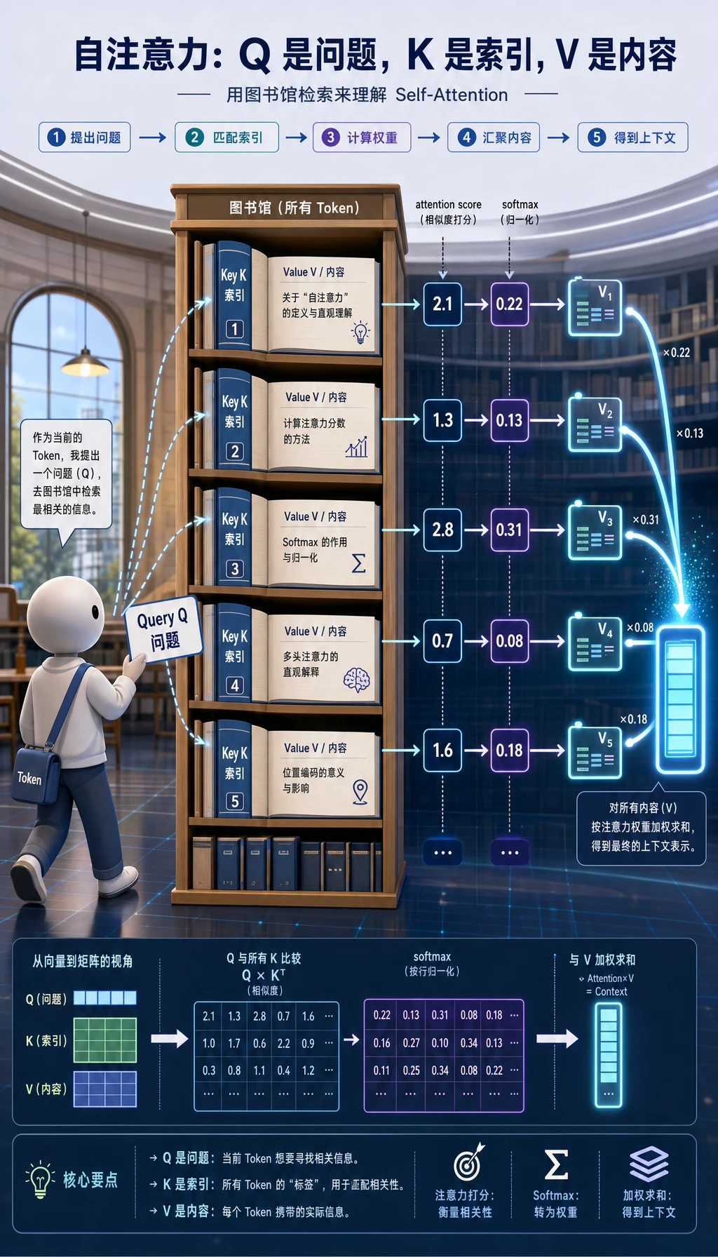
注意力是一种加权检索：

Q 提问→K 匹配→softmax 变成权重→V 提供内容→加权求和

检索类比：

角色	直觉	在注意力中
Query Q	我现在想找什么？	当前 token 的问题
Key K	每个条目匹配什么？	用来打分的索引
Value V	应该返回什么内容？	实际被混合的信息

一句话：

Q 和 K 打分，然后用得到的权重混合 V。

为什么需要注意力

旧式序列模型中，远处信息要么沿很多个循环步骤传递，要么被压进一个固定向量。注意力缩短了路径：

当前 token→直接给所有 token 打分→选择有用上下文

它带来三个实践优势：

• 直接建立长距离连接；
• 比一步步 RNN 更容易并行训练；
• 得到可观察的 token-to-token 混合权重矩阵。

实验 1：手算注意力

为了教学，令 Q = K = V = X。

import numpy as np

X = np.array(
    [
        [1.0, 0.0],
        [0.0, 1.0],
        [1.0, 1.0],
    ]
)

Q = K = V = X

scores = Q @ K.T
scaled_scores = scores / np.sqrt(K.shape[1])


def softmax(row):
    e = np.exp(row - row.max())
    return e / e.sum()


weights = np.apply_along_axis(softmax, 1, scaled_scores)
output = weights @ V

print("attention_lab")
print("scores")
print(np.round(scores, 3))
print("weights")
print(np.round(weights, 3))
print("output")
print(np.round(output, 3))

预期输出：

attention_lab
scores
[[1. 0. 1.]
 [0. 1. 1.]
 [1. 1. 2.]]
weights
[[0.401 0.198 0.401]
 [0.198 0.401 0.401]
 [0.248 0.248 0.503]]
output
[[0.802 0.599]
 [0.599 0.802]
 [0.752 0.752]]

读这三步：

步骤	代码	含义
打分	Q @ K.T	每个 token 和每个 token 有多匹配
归一化	softmax(...)	把分数变成和为 1 的权重
混合	weights @ V	按权重组合 token 内容

Lab 1B：Q/K/V 是学出来的视角，不是三份拷贝

手算实验里用了 Q = K = V = X，是为了让数学过程更容易看清。真实 Transformer 通常会学习三组投影矩阵：

Q = XW_q
K = XW_k
V = XW_v

这表示同一个 token 表示会被看成三种视角：

• Q：这个位置想找什么；
• K：这个位置提供什么匹配线索；
• V：如果被选中，这个位置贡献什么内容。

运行这个小版本：

import numpy as np

X = np.array(
    [
        [1.0, 0.0],
        [0.0, 1.0],
        [1.0, 1.0],
    ]
)

W_q = np.array([[1.0, 0.5], [0.0, 1.0]])
W_k = np.array([[0.5, 1.0], [1.0, 0.0]])
W_v = np.array([[1.0, -0.5], [0.5, 1.0]])

Q = X @ W_q
K = X @ W_k
V = X @ W_v

scores = Q @ K.T / np.sqrt(Q.shape[1])


def softmax(row):
    e = np.exp(row - row.max())
    return e / e.sum()


weights = np.apply_along_axis(softmax, 1, scores)
output = weights @ V

print("projection_lab")
for name, value in [("Q", Q), ("K", K), ("V", V), ("weights", weights), ("output", output)]:
    print(name)
    print(np.round(value, 3))

预期输出：

projection_lab
Q
[[1.  0.5]
 [0.  1. ]
 [1.  1.5]]
K
[[0.5 1. ]
 [1.  0. ]
 [1.5 1. ]]
V
[[ 1.  -0.5]
 [ 0.5  1. ]
 [ 1.5  0.5]]
weights
[[0.248 0.248 0.503]
 [0.401 0.198 0.401]
 [0.284 0.14  0.576]]
output
[[1.128 0.376]
 [1.102 0.198]
 [1.218 0.286]]

读证据：

• Q、K、V 来自同一个 X，但现在已经不同。
• 注意力权重由 Q 和 K 计算出来。
• 最终输出混合的是 V，不是原始的 X。

这就是为什么不要把 Q/K/V 只背成三个变量名。它们是三种学出来的视角，把匹配和内容混合分开。

留下的证据

保留一条 attention trace：

评分规则

Q @ K.T / sqrt(d_k)

权重规则

softmax 将分数转成每行和为 1 的行

输出规则

权重 @ V 混合 value 向量

QKV 规则

Q/K 决定匹配，V 携带内容

mask 规则

被屏蔽的位置获得接近 0 的注意力

LLM 桥接

因果注意力只允许生成使用过去的 token

为什么要除以 sqrt(d_k)？

Transformer 里的公式是：

Attention(Q, K, V) = softmax(QK^T / sqrt(d_k))V

当向量维度很大时，点积也容易变大。大分数会让 softmax 过于尖锐，某个 token 几乎拿走全部权重。除以 sqrt(d_k) 可以给分数降温，让训练更稳定。

Self-Attention

Self-attention 指 Q、K、V 都来自同一个序列。每个 token 都能看同一个序列里的每个 token。

例子：

"Alex gave Sam the notebook because he trusted him."

要理解 “he” 和 “him”，当前 token 需要看其他 token。Self-attention 给了这种直接路径。

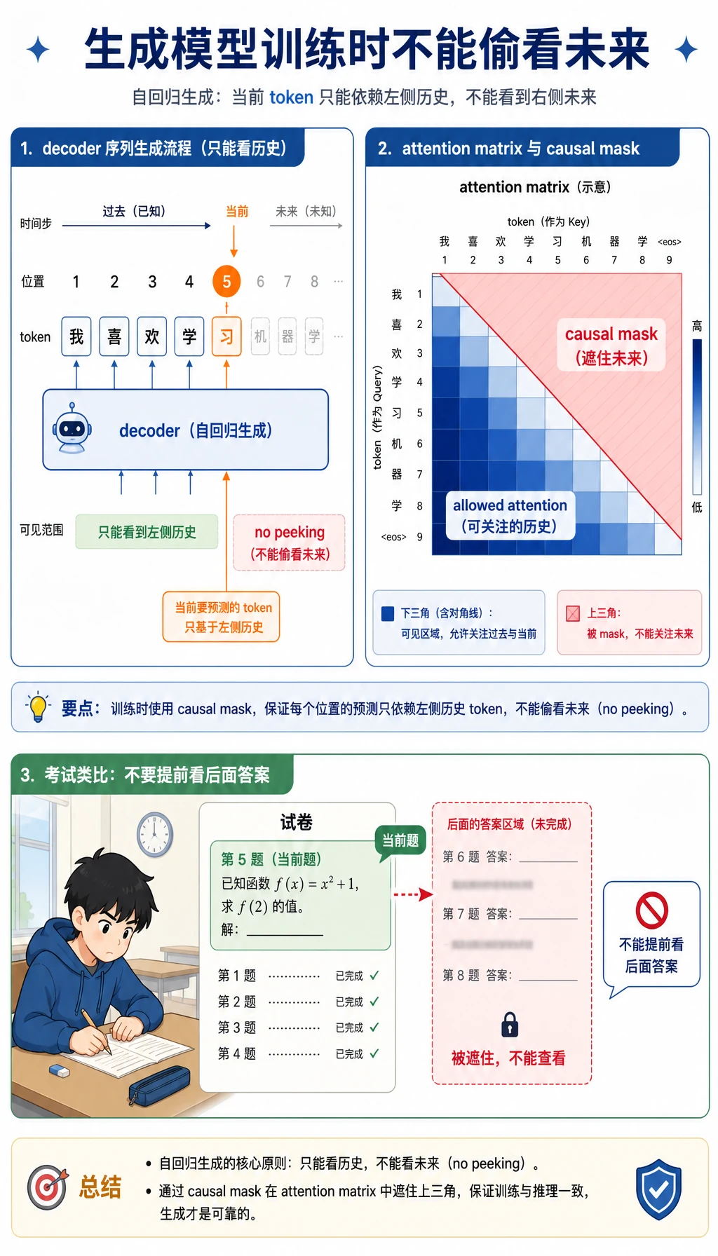
实验 2：Causal Mask

生成任务不能看未来 token。causal mask 只让下三角可见。

import numpy as np

scores = np.array(
    [
        [2.0, 1.0, 0.5],
        [1.2, 2.1, 0.7],
        [0.8, 1.3, 2.2],
    ]
)

mask = np.tril(np.ones_like(scores))
masked_scores = np.where(mask == 1, scores, -1e9)


def softmax(row):
    e = np.exp(row - row.max())
    return e / e.sum()


weights = np.apply_along_axis(softmax, 1, masked_scores)

print("mask_lab")
print(np.round(weights, 3))

预期输出：

mask_lab
[[1.    0.    0.   ]
 [0.289 0.711 0.   ]
 [0.149 0.246 0.605]]

读法：

• 位置 1 只能看自己；
• 位置 2 能看位置 1 和 2；
• 位置 3 能看位置 1、2、3。

未来答案不可见。

Multi-Head Attention

一个 attention head 可能只学到一种关系。multi-head attention 让模型并行查看多个关系空间。

不同 head 可能关注：

• 附近位置模式；
• 主语 / 宾语关系；
• 重复词；
• 长距离引用。

多个 head 的结果会拼接，再投影回一个表示。

实验 3：PyTorch MultiheadAttention

import torch
from torch import nn

torch.manual_seed(42)

attention = nn.MultiheadAttention(embed_dim=8, num_heads=2, batch_first=True)
tokens = torch.randn(1, 4, 8)
output, weights = attention(tokens, tokens, tokens)

print("mha_lab")
print("tokens:", tuple(tokens.shape))
print("output:", tuple(output.shape))
print("weights:", tuple(weights.shape))
print("row0_sum:", round(float(weights[0, 0].sum().detach()), 4))

预期输出：

mha_lab
tokens: (1, 4, 8)
output: (1, 4, 8)
weights: (1, 4, 4)
row0_sum: 1.0

shape 读法：

Tensor	Shape	含义
tokens	[1, 4, 8]	batch 1，4 个 token，embedding size 8
output	[1, 4, 8]	每个 token 得到新的上下文表示
weights	[1, 4, 4]	每个 query token 对 4 个 key token 分配权重

Attention 权重不是完整解释

Attention 权重很有用，但不要过度解读。

它能说明：

在这一层 / 这个 head 中，这个 query 从那些 key 位置混合了更多 value

它不能自动证明：

模型最终决策就是因为那个 token

把 attention 权重当作调试和观察工具，而不是完整因果解释。

常见错误

错误	修复
把 Q/K/V 当神秘变量	读成 问题 / 索引 / 内容
忘记 shape 含义	追踪 [batch, seq_len, embed_dim] 和 attention [batch, query, key]
生成任务不用 mask	用 causal mask 隐藏未来 token
在错误维度上 softmax	应该在 key 位置上归一化
把 attention 当推理魔法	记住：打分 -> softmax -> 加权求和

练习

1. 把实验 1 的第三个 token 改成 [2.0, 0.0]，weights 怎么变？
2. 在 Lab 1B 中，只修改 W_v。哪些打印值会变，哪些会保持不变？
3. 把 mask 实验扩展成 4 x 4 矩阵。
4. 把实验 3 的 num_heads 从 2 改成 1，哪些 shape 不变？
5. 解释为什么 attention 比普通 RNN 更容易建模远距离 token 交互。
6. 描述一个 attention 权重有帮助但不是完整解释的场景。

参考实现与讲解

1. 第三个 token 会更接近第一维方向的 query，因此这些 query 对它的 attention weight 通常会升高。精确数值取决于完整的 dot-product 表。
2. 只改 W_v 会改变 value vectors 和最终 attention output；attention scores 和 weights 不变，因为它们由 queries 和 keys 决定。
3. 4 x 4 causal mask 应允许每个位置看见自己和之前的位置，同时挡住未来位置。
4. 最终输出 shape 仍应是 [batch, seq, embed_dim]。变化的是模型如何把 embedding dimension 分给不同 heads。
5. Attention 让每个 token 都能直接访问所有可见 token；普通 RNN 需要把信息沿着很多顺序步骤传递，长距离信息更容易衰减。
6. Attention weights 可以提示某一层更关注哪些 token，但它不是完整解释，因为 value projection、residual path、后续层和 output head 都会继续影响最终答案。

小结

• Attention 让 token 直接选择相关上下文。
• Q/K/V 是学出来的视角，把匹配和内容检索分开。
• Scaled dot-product attention 是打分、softmax、加权求和。
• Causal mask 防止生成任务偷看未来。
• Multi-head attention 从多个子空间查看关系。