3.2.4 Array Operations

Learning Objectives

• Understand the concept and advantages of vectorized operations
• Master element-wise operations and universal functions (ufuncs)
• Understand the rules of Broadcasting
• Use aggregation functions confidently for statistical calculations

---

Vectorized Operations: Say Goodbye to Loops

Vectorized operations are a core idea in NumPy — operate on the entire array without writing loops.

Pure Python vs NumPy

import numpy as np

# Pure Python: compute one by one
prices = [100, 200, 300, 400, 500]
discounted = []
for p in prices:
    discounted.append(p * 0.8)
print(discounted)  # [80.0, 160.0, 240.0, 320.0, 400.0]

# NumPy: one line does it all
prices = np.array([100, 200, 300, 400, 500])
discounted = prices * 0.8
print(discounted)  # [ 80. 160. 240. 320. 400.]

Element-wise Operations

Arithmetic operations on NumPy arrays are performed element by element:

a = np.array([1, 2, 3, 4])
b = np.array([10, 20, 30, 40])

print(a + b)     # [11 22 33 44]    add corresponding elements
print(a - b)     # [ -9 -18 -27 -36]
print(a * b)     # [ 10  40  90 160]  multiply corresponding elements (not matrix multiplication!)
print(a / b)     # [0.1 0.1 0.1 0.1]
print(a ** 2)    # [ 1  4  9 16]      square
print(b % 3)     # [1 2 0 1]          remainder
print(b // 3)    # [ 3  6 10 13]      integer division

Operations with Scalars

When an array is operated on with a single number (a scalar), NumPy automatically applies the scalar to every element:

arr = np.array([10, 20, 30, 40])

print(arr + 5)    # [15 25 35 45]
print(arr * 2)    # [20 40 60 80]
print(arr / 10)   # [1. 2. 3. 4.]
print(1 / arr)    # [0.1  0.05 0.033 0.025]

Comparison Operations

arr = np.array([15, 23, 8, 42, 31])

print(arr > 20)      # [False  True False  True  True]
print(arr == 23)     # [False  True False False False]
print(arr != 8)      # [ True  True False  True  True]

---

Universal Functions (ufuncs)

NumPy provides many universal functions that apply mathematical operations to each element in an array:

Common Mathematical Functions

arr = np.array([1, 4, 9, 16, 25])

# Square root
print(np.sqrt(arr))     # [1. 2. 3. 4. 5.]

# Absolute value
neg = np.array([-3, -1, 0, 2, 5])
print(np.abs(neg))      # [3 1 0 2 5]

# Power
print(np.power(arr, 0.5))  # same as sqrt

# Exponential and logarithms
print(np.exp([0, 1, 2]))      # [1.    2.718 7.389]  e raised to a power
print(np.log([1, np.e, 10]))   # [0.    1.    2.303]  natural logarithm
print(np.log10([1, 10, 100]))  # [0. 1. 2.]           base 10
print(np.log2([1, 2, 8, 64]))  # [0. 1. 3. 6.]       base 2

Trigonometric Functions

# Create angles from 0 to 2π
angles = np.linspace(0, 2 * np.pi, 5)  # [0, π/2, π, 3π/2, 2π]

print(np.sin(angles))  # [ 0.  1.  0. -1.  0.]  ← sine
print(np.cos(angles))  # [ 1.  0. -1.  0.  1.]  ← cosine

Rounding Functions

arr = np.array([1.2, 2.5, 3.7, -1.3, -2.8])

print(np.floor(arr))    # [ 1.  2.  3. -2. -3.]  round down
print(np.ceil(arr))     # [ 2.  3.  4. -1. -2.]  round up
print(np.round(arr))    # [ 1.  2.  4. -1. -3.]  round to nearest
print(np.trunc(arr))    # [ 1.  2.  3. -1. -2.]  truncate decimals

Operations Between Two Arrays

a = np.array([3, 5, 7, 9])
b = np.array([1, 4, 2, 8])

print(np.maximum(a, b))  # [3 5 7 9]   take the larger value at each position
print(np.minimum(a, b))  # [1 4 2 8]   take the smaller value at each position
print(np.where(a > b, a, b))  # same as maximum, but more flexible

---

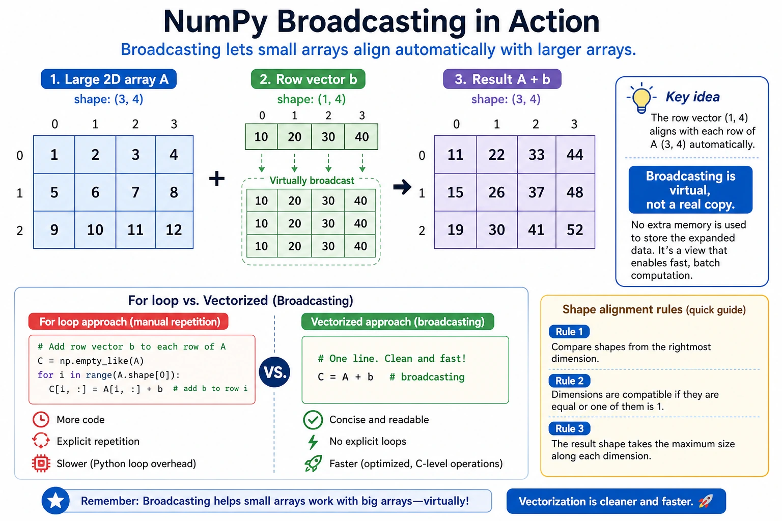
Broadcasting

When arrays with different shapes are operated on, NumPy automatically “broadcasts” the smaller array so their shapes become compatible.

The Simplest Example

arr = np.array([1, 2, 3])

# scalar + array → scalar is broadcast to [10, 10, 10]
print(arr + 10)   # [11 12 13]

This is broadcasting in action — NumPy expands 10 to [10, 10, 10], then adds element by element.

2D Array + 1D Array

matrix = np.array([
    [1, 2, 3],
    [4, 5, 6],
    [7, 8, 9]
])

row = np.array([10, 20, 30])

# row is broadcast to every row
result = matrix + row
print(result)
# [[11 22 33]
#  [14 25 36]
#  [17 28 39]]

You can think about broadcasting like this:

matrix:         row (before broadcasting):      row (after broadcasting):
[[1, 2, 3],    [10, 20, 30]  →   [[10, 20, 30],
 [4, 5, 6],                        [10, 20, 30],
 [7, 8, 9]]                        [10, 20, 30]]

Column Vector + Row Vector

col = np.array([[1], [2], [3]])    # shape: (3, 1) column vector
row = np.array([10, 20, 30])       # shape: (3,)   row vector

# both are broadcast
result = col + row
print(result)
# [[11 21 31]
#  [12 22 32]
#  [13 23 33]]

Broadcasting Rules

flowchart TD
    A["Are the two array shapes different?"] -->|Yes| B["Align dimensions from the end"]
    B --> C{"Does each dimension satisfy:<br/>1. equal<br/>2. one of them is 1"}
    C -->|All satisfied| D["Broadcast succeeds ✅<br/>Dimensions of 1 are copied and expanded"]
    C -->|Any not satisfied| E["Broadcast fails ❌<br/>Raises ValueError"]
    A -->|No| F["Shapes are the same, operate directly"]

Simple rule to remember: Compare dimensions from back to front — they must either be equal, or one of them must be 1.

# ✅ Can broadcast
# (3, 4) + (4,)     → (3, 4)     the last dimension is 4 in both
# (3, 4) + (1, 4)   → (3, 4)     first dimension 3 and 1 → broadcast to 3
# (3, 1) + (1, 4)   → (3, 4)     both dimensions are broadcast

# ❌ Cannot broadcast
# (3, 4) + (3,)     → error! last dimension 4 ≠ 3, and neither is 1

Real-World Uses of Broadcasting

# Standardize data: subtract the mean of each column from that column
data = np.array([
    [85, 170, 60],
    [92, 180, 75],
    [78, 165, 55],
    [90, 175, 70]
])  # 4 students: score, height, weight

# Compute the mean of each column
col_mean = data.mean(axis=0)        # [86.25 172.5  65.  ]  shape: (3,)

# Broadcasting: (4, 3) - (3,) → (4, 3)
centered = data - col_mean
print(centered)
# [[-1.25 -2.5  -5.  ]
#  [ 5.75  7.5  10.  ]
#  [-8.25 -7.5 -10.  ]
#  [ 3.75  2.5   5.  ]]

---

Aggregation Functions

Aggregation functions “summarize” a group of data into one value or a small set of values:

Common Aggregation Functions

arr = np.array([4, 7, 2, 9, 1, 5, 8, 3, 6])

print(np.sum(arr))      # 45    total
print(np.mean(arr))     # 5.0   mean
print(np.median(arr))   # 5.0   median
print(np.std(arr))      # 2.58  standard deviation
print(np.var(arr))      # 6.67  variance
print(np.min(arr))      # 1     minimum
print(np.max(arr))      # 9     maximum
print(np.argmin(arr))   # 4     index of minimum
print(np.argmax(arr))   # 3     index of maximum
print(np.cumsum(arr))   # [ 4 11 13 22 23 28 36 39 45]  cumulative sum
print(np.cumprod(arr[:5]))  # [  4  28  56 504 504]  cumulative product

Aggregation Along an Axis

For multi-dimensional arrays, the axis parameter controls which direction to aggregate along:

matrix = np.array([
    [1, 2, 3],
    [4, 5, 6],
    [7, 8, 9]
])

# No axis specified: aggregate all elements
print(np.sum(matrix))          # 45

# axis=0: along the row direction (aggregate by column) — compress top to bottom
print(np.sum(matrix, axis=0))  # [12 15 18]

# axis=1: along the column direction (aggregate by row) — compress left to right
print(np.sum(matrix, axis=1))  # [ 6 15 24]

A helpful way to understand axis — axis=0 removes rows, axis=1 removes columns:

Axis	Mental model	Result
axis=0	compress top to bottom, keep columns	[12, 15, 18]
axis=1	compress left to right, keep rows	[6, 15, 24]

If you are unsure, print matrix.shape first, then ask which dimension you want to remove.

Practice: Grade Analysis

# Scores for 5 students in 3 subjects
scores = np.array([
    [85, 92, 78],   # Student 1: Chinese, Math, English
    [90, 88, 95],   # Student 2
    [72, 65, 80],   # Student 3
    [95, 98, 92],   # Student 4
    [60, 55, 70]    # Student 5
])

subjects = ["Chinese", "Math", "English"]

# Total score for each student
total = np.sum(scores, axis=1)
print("Total score for each student:", total)   # [255 273 217 285 185]

# Average score for each student
avg_per_student = np.mean(scores, axis=1)
print("Average score for each student:", avg_per_student)

# Average score for each subject
avg_per_subject = np.mean(scores, axis=0)
for sub, avg in zip(subjects, avg_per_subject):
    print(f"  {sub} average score: {avg:.1f}")

# Who got the highest score, and in which subject
max_idx = np.unravel_index(np.argmax(scores), scores.shape)
print(f"Highest score: {scores[max_idx]} (Student {max_idx[0]+1}'s {subjects[max_idx[1]]})")

# Which student has the highest total score
best_student = np.argmax(total)
print(f"Highest total score: Student {best_student + 1}, total {total[best_student]}")

---

np.where: Conditional Selection

np.where is NumPy’s version of the ternary expression:

arr = np.array([85, 42, 91, 67, 55, 78])

# Mark passing scores as "PASS" and failing scores as "FAIL"
result = np.where(arr >= 60, "PASS", "FAIL")
print(result)  # ['PASS' 'FAIL' 'PASS' 'PASS' 'FAIL' 'PASS']

# Raise failing scores to 60
adjusted = np.where(arr >= 60, arr, 60)
print(adjusted)  # [85 60 91 67 60 78]

---

Evidence to Keep

Keep this page’s proof of learning as a small evidence card:

Array State

shape, dtype, axis, and sample values before the operation

Operation

indexing, slicing, broadcasting, reshape, linear algebra, or random/stat function

Output

resulting array shape, values, or statistic

Failure Check

axis confusion, view/copy trap, broadcast mismatch, or wrong shape

Expected Output

printed shapes and values that make the array operation inspectable

Summary

Category	Content	Example
Vectorized operations	Operate on the whole array at once, no loops needed	arr * 2, a + b
Universal functions	Element-wise mathematical functions	np.sqrt(), np.exp(), np.log()
Broadcasting	Automatically expand arrays with different shapes	(3,4) + (4,) → (3,4)
Aggregation functions	Statistical summaries	np.sum(), np.mean(), np.std()
axis parameter	Controls aggregation direction	axis=0 by column, axis=1 by row
np.where	Conditional selection	np.where(arr > 0, arr, 0)

---

Hands-On Exercises

Exercise 1: Vectorized Calculation

# Convert Fahrenheit to Celsius
# Formula: C = (F - 32) × 5/9
import numpy as np

fahrenheit = np.array([32, 68, 100, 212, 72, 98.6])

# Complete the conversion in one line using vectorized operations
celsius = (fahrenheit - 32) * 5 / 9

Exercise 2: Broadcasting Practice

# Original prices of 3 products
import numpy as np

prices = np.array([100, 200, 300])

# 3 discount rates (column vector)
discounts = np.array([[0.9], [0.8], [0.7]])

# Use broadcasting to calculate the price of each product under each discount (3×3 matrix)
final_prices = discounts * prices
# Expected result:
# [[ 90. 180. 270.]
#  [ 80. 160. 240.]
#  [ 70. 140. 210.]]

Exercise 3: Grade Statistics

# Generate random scores for 50 students (between 40 and 100)
rng = np.random.default_rng(seed=42)
scores = rng.integers(40, 101, size=50)

# 1. Compute the mean, median, and standard deviation
# 2. Find the highest score, lowest score, and their positions
# 3. Count how many students fall into each range: failing (<60), passing (60-69), average (70-79), good (80-89), excellent (90+)
# 4. Calculate the passing rate

Reference implementation and walkthrough

• Fahrenheit to Celsius should use (fahrenheit - 32) * 5 / 9; the given examples produce about [0, 20, 37.78, 100, 22.22, 37].
• Broadcasting works when NumPy can align dimensions from the right. In the common row-plus-column exercise, the result becomes a 3 by 3 matrix because each row value combines with each column value.
• For score statistics, report mean, median, standard deviation, highest and lowest index or name, pass rate, and a bin count. The explanation should use array operations, not a manual loop.