5.5.4 Feature Construction

Section Overview

Feature construction is about creating new features from existing data. It is often the most effective way to improve model performance. In Kaggle competitions, the winner is often decided by who built better features.

Learning Objectives

• Master polynomial features and interaction features
• Master time feature extraction
• Master statistical features (group statistics)
• Understand domain-knowledge-driven feature design

---

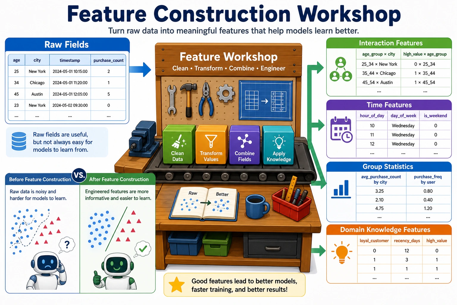
First, Build a Map

Feature construction is not about “randomly creating more columns” — it is:

Turning raw fields into representations that are closer to the essence of the problem.

flowchart LR
    A["Raw Fields"] --> B["Combination"]
    A --> C["Transformation"]
    A --> D["Group Statistics"]
    A --> E["Domain-Knowledge Derivation"]
    B --> F["New Features"]
    C --> F
    D --> F
    E --> F

A Better Analogy for Beginners

You can think of feature construction as:

• Processing raw materials into semi-finished products that are more suitable for model input

Raw fields are often like:

• Vegetables that have not been cut yet

Constructed features are more like:

• Ingredients that have already been cut and prepared for a specific use, ready to go into the pan

So the real point of feature construction is not to “create a few more columns,” but to:

• make the data closer to the essence of the problem

When Is Feature Construction Worth Doing?

• The raw fields are too “raw,” and the model cannot easily learn the relationship
• You have already found some combination patterns in EDA
• The business clearly has more natural derived metrics

When Should You Not Create Features Carelessly?

• You have not yet understood the raw features themselves
• The new feature is only there to “look more complicated”
• You already have many features but have not done selection or validation

A Construction Order Beginners Can Follow Directly

A more stable order is usually:

1. Start with the most natural business ratios or differences
2. Then add a small number of interaction features
3. Then look at time features and group statistics
4. Only then consider more aggressive automatic combinations

This is usually easier than piling on polynomial features from the start, because it makes it clearer where the gains come from.

Polynomial Features and Interaction Features

from sklearn.preprocessing import PolynomialFeatures
import numpy as np
import pandas as pd

# Raw features
X = np.array([[2, 3], [4, 5]])
feature_names = ['x1', 'x2']

# Second-order polynomial features (including interaction terms)
poly = PolynomialFeatures(degree=2, include_bias=False)
X_poly = poly.fit_transform(X)
print("Raw features:", feature_names)
print("Polynomial features:", poly.get_feature_names_out(feature_names))
print(f"Number of features: {X.shape[1]} → {X_poly.shape[1]}")

Raw	Generated	Explanation
x1, x2	x1², x2²	Quadratic terms
x1, x2	x1×x2	Interaction term

Note

Polynomial features can cause the number of features to explode. A 3rd-degree polynomial with 10 features will produce 286 features. Usually, use degree=2 and combine it with feature selection.

When You First Learn Interaction Features, What Is Most Worth Remembering?

What is most worth remembering is not the formula, but:

• some relationships cannot be expressed by a single field

For example:

• Housing prices depend not only on area
• They may also depend on combinations such as “area × location”

So interaction features are essentially asking:

• If we combine two factors, is the result more informative than looking at either one alone?

---

Time Feature Extraction

# Extract rich features from dates
dates = pd.date_range('2024-01-01', periods=100, freq='D')
df_time = pd.DataFrame({'date': dates})

df_time['year'] = df_time['date'].dt.year
df_time['month'] = df_time['date'].dt.month
df_time['day'] = df_time['date'].dt.day
df_time['dayofweek'] = df_time['date'].dt.dayofweek     # 0=Monday, 6=Sunday
df_time['is_weekend'] = df_time['dayofweek'].isin([5, 6]).astype(int)
df_time['quarter'] = df_time['date'].dt.quarter
df_time['day_of_year'] = df_time['date'].dt.dayofyear

print(df_time.head(10))

Extracted Feature	Use Case
Year / month / day	Trends and seasonality
Day of week / weekend or not	Differences in consumer behavior
Hour / minute	Intra-day patterns
Quarter	Quarterly business analysis
Days from an event	Holiday effects

A Beginner-Friendly Rule of Thumb

Time fields are often not “just one field,” but a bundle of hidden patterns:

• cycles
• rhythms
• distance from an event

So what we most often do with time features is not only extract year/month/day, but also break “when” into “cycle and position.”

---

Statistical Features (Group Statistics)

import seaborn as sns

df = sns.load_dataset('tips')

# Group-based statistical features
df['avg_tip_by_day'] = df.groupby('day')['tip'].transform('mean')
df['max_bill_by_time'] = df.groupby('time')['total_bill'].transform('max')
df['tip_pct'] = df['tip'] / df['total_bill']
df['bill_rank_in_day'] = df.groupby('day')['total_bill'].rank(pct=True)

print(df[['day', 'total_bill', 'tip', 'avg_tip_by_day', 'tip_pct', 'bill_rank_in_day']].head(10))

Statistic Type	Example	Scenario
Group mean	Average spending per day	Comparison within the same group
Group count	Number of orders per user	Activity level
Rank/percentile	Spending rank within the group	Relative position
Difference/ratio	Tip/bill ratio	Derived metric

Another Minimal Example of “Relative Position Within the Same Group”

df_small = pd.DataFrame({
    "city": ["A", "A", "A", "B", "B"],
    "income": [10, 20, 30, 5, 15],
})

df_small["city_mean_income"] = df_small.groupby("city")["income"].transform("mean")
df_small["income_minus_city_mean"] = df_small["income"] - df_small["city_mean_income"]

print(df_small)

This example is especially good for beginners because it helps you first see that:

• sometimes absolute values are not enough
• “Is it high or low in its own group?” matters more

---

Domain-Knowledge-Driven Feature Design

Good features often come from understanding the business:

Domain	Raw Features	Constructed Feature
E-commerce	Total spending, number of orders	Average order value = total spending / number of orders
Real estate	Area, number of rooms	Area per room = area / number of rooms
Finance	Income, debt	Debt ratio = debt / income
User	Registration time, last login	Days of inactivity = today - last login

# Example of domain features for housing data
rng = np.random.default_rng(seed=42)
house = pd.DataFrame({
    'area': rng.uniform(50, 200, 100),
    'rooms': rng.integers(1, 6, 100),
    'floor': rng.integers(1, 30, 100),
    'age': rng.integers(0, 30, 100),
})

# Domain features
house['area_per_room'] = house['area'] / house['rooms']
house['is_new'] = (house['age'] <= 5).astype(int)
house['is_high_floor'] = (house['floor'] >= 15).astype(int)

print(house.head())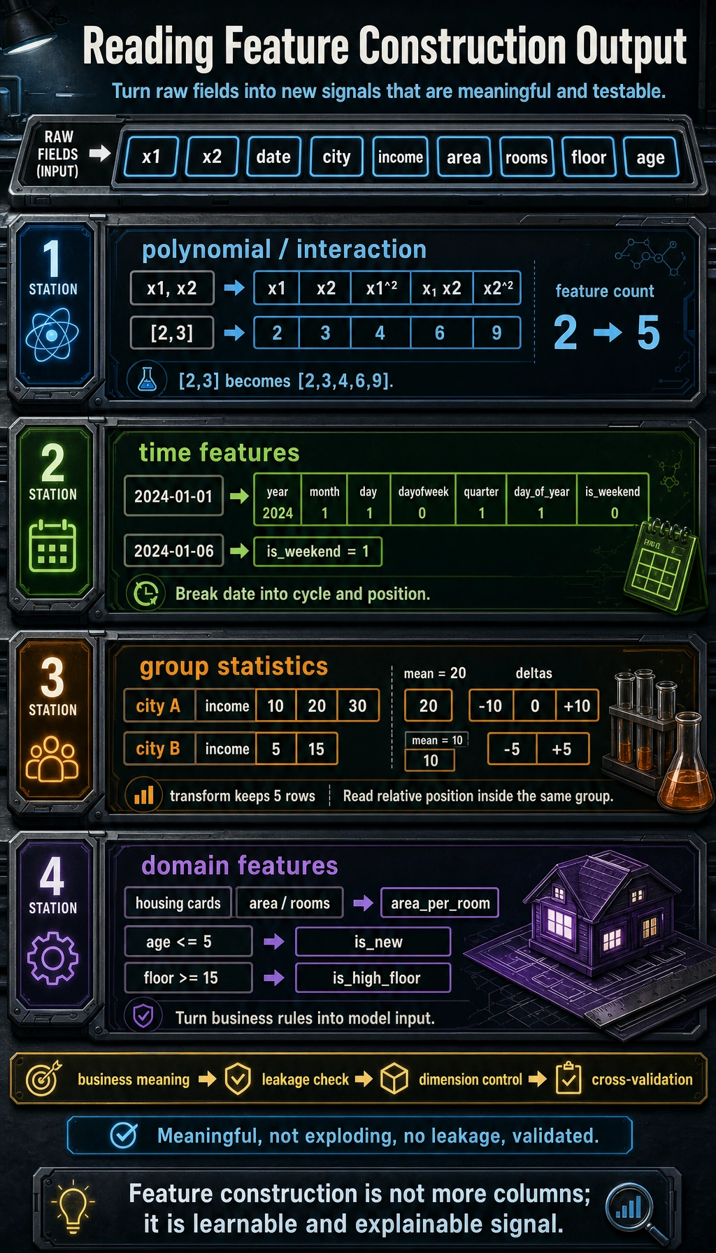

Read constructed features as evidence

A useful constructed feature should have a clear meaning, avoid leakage, keep dimensionality under control, and improve validation results before you keep it.

Why Are Domain-Knowledge Features Often the Most Valuable?

Because they are often closest to the metrics the business really cares about. For example:

• real estate focuses on “area per room”
• e-commerce focuses on “average order value”
• finance focuses on “debt ratio”

These features often look more like decision variables than the raw fields themselves.

---

Don’t Forget These Three Things After Feature Construction

1. Check whether the dimensionality has exploded
2. Check whether cross-validation scores actually improved
3. Check whether the new features make the model harder to explain or easier to leak information

A Feature Construction Checklist Beginners Can Copy Directly

When you build features for the first time, the safest checklist is usually:

1. Does this new feature have a clear business meaning?
2. Is it too directly related to the target variable, creating leakage risk?
3. Did cross-validation really improve after adding it?
4. If it improved, can I explain why?

If you cannot answer these four questions clearly, the feature usually is not worth keeping right away.

If You Put This Section Into a Project, What Is Most Worth Showing?

• A comparison between the raw features and the new features
• Why the new features make business sense
• A score comparison between the baseline and the model with added features
• One or two examples showing that the new features really helped the model

---

Evidence to Keep

Keep this page’s proof of learning as a small evidence card:

Feature State

raw columns, types, missing values, scale, and target relationship

Transformation

preprocessing, construction, selection, or pipeline step

Output

transformed feature table, pipeline object, score change, or selected features

Failure Check

leakage, inconsistent train/test transform, high-cardinality trap, or meaningless feature

Expected Output

feature pipeline evidence with before/after and metric impact

Summary

Method	Description	Key Point
Polynomial / interaction	Automatically generate higher-order and combined features	Watch out for feature explosion
Time features	Extract cyclical information from dates	Day of week, month, holiday or not
Statistical features	Use group aggregation to create relative indicators	transform keeps the row count unchanged
Domain knowledge	Construct features based on business understanding	Most effective, but depends on experience

Hands-on Exercises

Exercise 1: Titanic Feature Construction

On the Titanic dataset, construct: family size (sibsp + parch + 1), whether the passenger traveled alone, fare bands, and titles in names. Observe the improvement in model performance.

Exercise 2: Time Series Features

Generate one year of date data, extract all time features (month, week, quarter, whether it is a working day), and use bar charts to show the distribution of different features.

Solution approach and explanation

1. Titanic features should be compared against a baseline with the same split and model. Useful new features often improve validation score modestly and make business sense, such as family size capturing travel context.
2. Fare bands and titles must be created inside the training workflow if they learn cut points or mappings. Avoid using the full dataset to choose bins that indirectly depend on test distribution.
3. Time features should reveal seasonality or calendar effects. Month, week, quarter, weekday, weekend, and holiday flags are useful only if the target plausibly changes with time.
4. A good answer includes before/after metrics, a short reason for each feature, and at least one feature that was rejected because it was noisy, redundant, or unavailable in production.