4.1.5 Vector Spaces and Linear Transformations [Elective]

Elective Chapter

This section is here to help you build deeper understanding. If you just want to get started quickly with AI projects, you can skip it for now and come back later when you encounter these concepts again.

Learning Objectives

• Understand the meaning of linear independence, basis, and dimension
• Understand the matrix representation of linear transformations
• Build intuition for singular value decomposition (SVD)

First, let’s set an important learning expectation

This section is elective, and the title is more abstract, so beginners often slow down right away. Your most important goal here is not to fully master every advanced theory in linear algebra, but to first build a higher-level perspective:

• What the vectors, matrices, and eigenvalues from earlier sections really are in the bigger picture
• Why terms like “dimension,” “basis,” and “linear independence” keep showing up later in AI
• Why SVD becomes a foundational tool in many methods

In other words, this section is more like:

A higher-level framework that organizes the intuition from the previous three sections.

---

How does this section relate to the previous three?

If the previous three sections were about “how vectors are represented, how matrices transform, and how eigenvalues find special directions,” then this section raises the viewpoint and looks at all of that again from a broader angle.

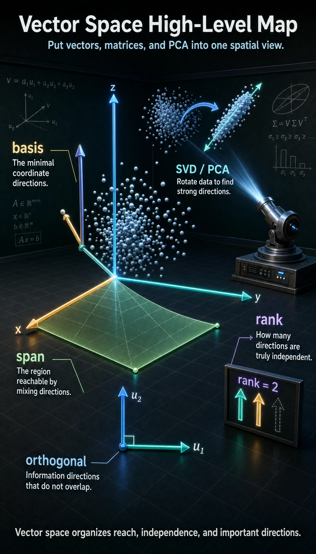
So this lesson is more like a “deeper understanding and organization” lesson. You do not need to fully master it right away, but once you do understand it, you will better see why the earlier concepts make sense.

Acronyms and Notation to Decode Before Going Deeper

Term	Full name	Beginner-friendly meaning
SVD	Singular Value Decomposition	Split a matrix into directions, strengths, and reconstruction steps
PCA	Principal Component Analysis	Find the most important directions in data and keep fewer dimensions
NLP	Natural Language Processing	AI methods for text and language
LSA	Latent Semantic Analysis	A classic text method that uses SVD to find hidden topic structure
V^T / Vt	V transpose	Flip rows and columns of V; NumPy often names it Vt
rank	Matrix rank	How many independent directions a matrix really contains
basis	Basis vectors	A minimal set of non-redundant coordinate directions
span	Span of vectors	Everything you can reach by mixing the given vectors
orthogonal	Perpendicular / independent directions	Directions that do not overlap; in AI this often means cleaner separation of information
full_matrices=False	Compact SVD mode	Ask NumPy to return only the useful part of U and Vt, so reconstruction shapes are easier to multiply
np.linalg	NumPy linear algebra module	The part of NumPy that contains matrix tools such as rank, solve, eigenvalues, and SVD
Low-rank approximation	Approximation with fewer effective dimensions	Keep only the most important singular values and drop weaker details

Code setup for this lesson: the snippets are written in a notebook style. If you run them in order, the later blocks can reuse np, plt, and variables defined earlier. If you copy one block into a fresh .py file, add these imports first:

import numpy as np
import matplotlib.pyplot as plt

np is the standard short alias for NumPy, the Python library for arrays and linear algebra. plt is the common alias for Matplotlib pyplot, the plotting tool used for diagrams.

Linear Independence — Vectors with “No Redundancy”

What is linear independence?

Intuition: A set of vectors is “linearly independent” if each vector contributes unique information, and none of them is unnecessary.

A beginner-friendly analogy

You can think of “linear independence” like team roles:

• If everyone on the team brings a different ability, then there is no redundancy
• If two people are doing the same thing, then one of them is somewhat repeated

So the most important thing to remember about linear independence is not the formal definition, but this sentence:

In this set of vectors, is anyone just repeating information that someone else has already expressed?

import numpy as np
import matplotlib.pyplot as plt

plt.rcParams['font.sans-serif'] = ['Arial Unicode MS']
plt.rcParams['axes.unicode_minus'] = False

# Example of linear independence: right and up, completely different directions
v1 = np.array([1, 0])
v2 = np.array([0, 1])

# Example of linear dependence: v2 is just 2 times v1, same direction
u1 = np.array([1, 2])
u2 = np.array([2, 4])  # u2 = 2 * u1, redundant!

fig, axes = plt.subplots(1, 2, figsize=(12, 5))

# Linear independence
ax = axes[0]
ax.quiver(0, 0, v1[0], v1[1], angles='xy', scale_units='xy', scale=1,
          color='steelblue', width=0.01, label='v1 = [1, 0]')
ax.quiver(0, 0, v2[0], v2[1], angles='xy', scale_units='xy', scale=1,
          color='coral', width=0.01, label='v2 = [0, 1]')
ax.set_xlim(-0.5, 2)
ax.set_ylim(-0.5, 2)
ax.set_aspect('equal')
ax.grid(True, alpha=0.3)
ax.legend()
ax.set_title('Linear independence\nTwo different directions, no redundancy')

# Linear dependence
ax = axes[1]
ax.quiver(0, 0, u1[0], u1[1], angles='xy', scale_units='xy', scale=1,
          color='steelblue', width=0.01, label='u1 = [1, 2]')
ax.quiver(0, 0, u2[0], u2[1], angles='xy', scale_units='xy', scale=1,
          color='coral', width=0.01, label='u2 = [2, 4]')
ax.set_xlim(-0.5, 3)
ax.set_ylim(-0.5, 5)
ax.set_aspect('equal')
ax.grid(True, alpha=0.3)
ax.legend()
ax.set_title('Linear dependence\nu2 = 2×u1, completely redundant')

plt.tight_layout()
plt.show()

Why this matters in AI

Scenario	Why linear independence matters
Feature engineering	If two features are linearly dependent (for example, “temperature (°C)” and “temperature (°F)”), one of them is redundant
PCA dimensionality reduction	Principal components are orthogonal to each other (linearly independent), and each one provides unique information
Neural networks	If the columns of a weight matrix are linearly dependent, it means some neurons are redundant

Using matrix rank to judge it

Matrix rank = the maximum number of linearly independent rows (or columns) in a matrix.

# 3 columns are linearly independent
A = np.array([[1, 0, 0],
              [0, 1, 0],
              [0, 0, 1]])
print(f"Rank of A: {np.linalg.matrix_rank(A)}")  # 3 (full rank)

# The 3rd column = the 1st column + the 2nd column, redundant!
B = np.array([[1, 0, 1],
              [0, 1, 1],
              [0, 0, 0]])
print(f"Rank of B: {np.linalg.matrix_rank(B)}")  # 2 (not full rank)

Expected output:

Rank of A: 3
Rank of B: 2

Here, “full rank” means no column is wasted. Matrix B has three columns, but only two independent directions, so its effective information dimension is 2.

---

Basis and Dimension — the “Coordinate System” of a Space

Basis

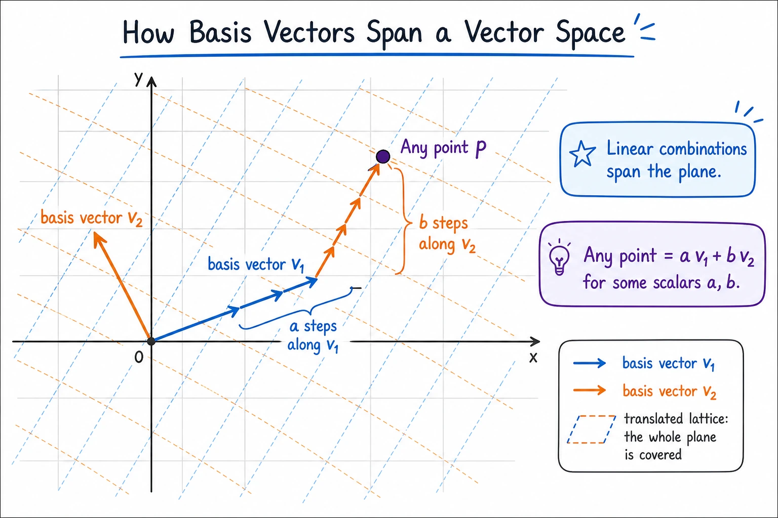
A basis = a set of linearly independent vectors that can “span” the entire space (that is, any vector can be expressed as a combination of them).

The most important thing to remember about a basis is not the term, but its role

You can think of a basis as:

• A minimal, sufficient, and non-redundant coordinate system

In other words:

• It can represent everything you need
• It does not contain extra directions

This is exactly why many AI methods are always looking for a “better basis for representation.”

The most common basis is the standard basis:

# Standard basis in 2D space
e1 = np.array([1, 0])  # x direction
e2 = np.array([0, 1])  # y direction

# Any 2D vector can be represented using the standard basis
v = np.array([3, 5])
# v = 3 * e1 + 5 * e2

print(f"v = {v[0]} × e1 + {v[1]} × e2 = {v[0]*e1 + v[1]*e2}")

Expected output:

v = 3 × e1 + 5 × e2 = [3 5]

A non-standard basis also works:

# Change to another basis
b1 = np.array([1, 1])
b2 = np.array([1, -1])

# What are the coordinates of v = [3, 5] in the new basis?
# v = c1 * b1 + c2 * b2
# Solve the system of equations
B = np.column_stack([b1, b2])
coords = np.linalg.solve(B, v)
print(f"Coordinates in the new basis: {coords}")  # [4, -1]
# Check: 4*[1,1] + (-1)*[1,-1] = [4,4]+[-1,1] = [3,5] ✓

Expected output:

Coordinates in the new basis: [ 4. -1.]

This is the key idea: the vector did not move, but its coordinates changed because we described it using a different coordinate system. This is why “representation” is such a big word in AI.

Dimension

Dimension = the number of basis vectors = the minimum number of coordinates needed to describe a space.

Why does “dimension” become such a frequent term in AI?

Because in AI, you often care about two things:

• How many degrees of freedom the current representation actually has
• Whether you can reduce the dimension while losing as little information as possible

So in AI, dimension is not just a geometric term. It often means:

• Computational cost
• Information capacity
• Model complexity

Space	Dimension	Example
A line	1	Temperature scale
A plane	2	Position on a map
3D space	3	Position in the real world
Word vector space	100~300	A word’s “semantic coordinates”
Image pixel space	tens of thousands to millions	Each pixel is a dimension

Dimensions in AI

In AI, people often say “high-dimensional space” — a 28×28 handwritten digit image is a point in a 784-dimensional space. The essence of PCA is to find a new set of “basis vectors” (principal components) so that we can use fewer dimensions (for example, 2D) to approximately represent the data.

---

Matrix Representation of Linear Transformations

A linear transformation = a matrix

A very deep result: any linear transformation can be represented by a matrix.

Why is this especially important for AI?

Because it unifies many things that seem different into the same form of expression:

• Rotation
• Scaling
• Projection
• A neural network layer

In other words, many “layers” in AI can be understood first as:

• Some linear transformation + subsequent nonlinear processing

What is a linear transformation? A transformation T that satisfies two conditions:

1. T(a + b) = T(a) + T(b) (addition can be “moved in and out”)
2. T(ka) = k·T(a) (scalar multiplication can be “moved in and out”)

# Rotation, scaling, projection, shearing... all are linear transformations

# Look at where the standard basis vectors go, and you know the matrix
# A 90° rotation:
# e1 = [1, 0] → [0, 1]
# e2 = [0, 1] → [-1, 0]

# Put the transformed basis vectors as columns, and you get the transformation matrix!
R90 = np.array([[0, -1],
                [1,  0]])

# Verify
print(R90 @ np.array([1, 0]))  # [0, 1] ✓
print(R90 @ np.array([0, 1]))  # [-1, 0] ✓

Expected output:

[0 1]
[-1  0]

The matrix is fully determined by where it sends the basis vectors. That is why a matrix is not just a table of numbers; it is a compact description of a transformation.

Composition of transformations = matrix multiplication

Rotate by 45° first, then scale by 2? Just multiply the two matrices.

# Rotate 45°
theta = np.radians(45)
R45 = np.array([
    [np.cos(theta), -np.sin(theta)],
    [np.sin(theta),  np.cos(theta)]
])

# Scale by 2
S2 = np.array([
    [2, 0],
    [0, 2]
])

# Rotate first, then scale = S2 @ R45 (note: read from right to left!)
combined = S2 @ R45
print(f"Combined transformation matrix:\n{combined.round(3)}")

# Apply to a vector
v = np.array([1, 0])
result = combined @ v
print(f"[1, 0] → {result.round(3)}")  # ≈ [1.414, 1.414]

Expected output:

Combined transformation matrix:
[[ 1.414 -1.414]
 [ 1.414  1.414]]
[1, 0] → [1.414 1.414]

Read S2 @ R45 @ v from right to left: the vector is rotated first, then scaled. This “rightmost operation happens first” rule also appears in neural network code when multiple matrix operations are chained.

---

SVD — the “Swiss Army Knife” of Matrix Decomposition

What is SVD?

Singular Value Decomposition (SVD) is a generalization of eigenvalue decomposition — it applies to matrices of any shape (not limited to square matrices).

A beginner-friendly analogy

You can think of SVD as:

• Breaking a complicated transformation into several smaller actions that are easier to understand

It is a lot like taking apart a machine to see how it works:

1. First, how it is oriented
2. Then, how it stretches
3. Finally, how it is rotated back toward the target direction

That is also why it becomes a foundational tool in many AI methods:

• Because it is not only something you can compute
• It is also very good for explaining structure

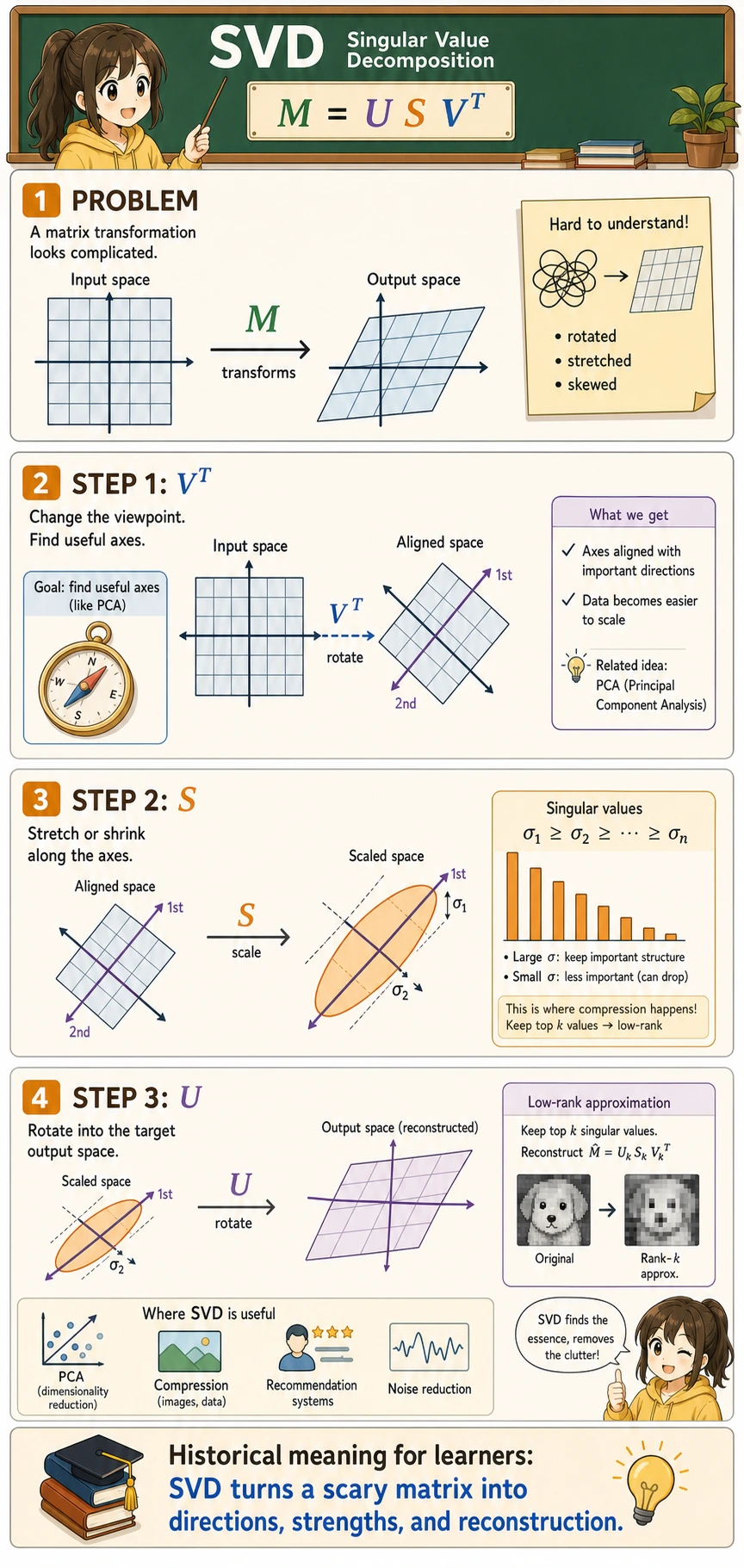
SVD decomposes a matrix M into the product of three matrices:

M = U × S × V^T

Where:

• U: left singular vectors (orthogonal matrix)
• S: singular values (diagonal matrix, sorted from large to small)
• V^T: V transpose, the transpose of the right singular vector matrix

In NumPy, np.linalg.svd() returns U, S, Vt. Notice that S is returned as a one-dimensional list of singular values, so when reconstructing the matrix you usually write np.diag(S) to turn it into a diagonal matrix.

full_matrices=False tells NumPy to return the compact form. For a beginner, this is usually the friendliest choice because the shapes line up directly:

• U: (rows, number_of_singular_values)
• np.diag(S): (number_of_singular_values, number_of_singular_values)
• Vt: (number_of_singular_values, columns)

# SVD of an arbitrary matrix
M = np.array([
    [1, 2, 3],
    [4, 5, 6],
])  # 2×3 matrix

U, S, Vt = np.linalg.svd(M, full_matrices=False)

print(f"Shape of U: {U.shape}")     # (2, 2)
print(f"Singular values S: {S.round(3)}")  # [9.508, 0.773]
print(f"Shape of Vt: {Vt.shape}")   # (2, 3)

# Verify: M ≈ U @ diag(S) @ Vt
reconstructed = U @ np.diag(S) @ Vt
print(f"\nReconstruction error: {np.linalg.norm(M - reconstructed):.10f}")  # ≈ 0

Expected output:

Shape of U: (2, 2)
Singular values S: [9.508 0.773]
Shape of Vt: (2, 3)

Reconstruction error: 0.0000000000

The first singular value is much larger than the second one, so the matrix has one very strong direction and one weaker correction direction. This “strong structure first, details later” idea is exactly why SVD is useful for compression and dimensionality reduction.

The intuition behind SVD

SVD decomposes any transformation into three steps:

flowchart LR
    A["Original space"] -->|"V transpose<br/>rotation"| B["Align with principal axes"]
    B -->|"S<br/>scale along axes"| C["After scaling"]
    C -->|"U<br/>rotate to target"| D["Target space"]

    style A fill:#e3f2fd,stroke:#1565c0,color:#333
    style B fill:#fff3e0,stroke:#e65100,color:#333
    style C fill:#fff3e0,stroke:#e65100,color:#333
    style D fill:#e8f5e9,stroke:#2e7d32,color:#333

An SVD application: image compression

The most intuitive application of SVD is using less data to approximate an image:

# Use a grayscale image as an example
# Here we use random numbers to simulate a grayscale image
rng = np.random.default_rng(seed=42)
image = rng.integers(0, 256, (100, 150)).astype(float)
# Add some structure (not pure randomness)
for i in range(100):
    for j in range(150):
        image[i, j] = 128 + 50 * np.sin(i/10) * np.cos(j/15) + rng.normal() * 20

print(f"Original image: {image.shape} = {image.size} values")

# SVD decomposition
U, S, Vt = np.linalg.svd(image, full_matrices=False)
print(f"Number of singular values: {len(S)}")

for k in [1, 5, 20, 100]:
    compressed_size = k * (U.shape[0] + 1 + Vt.shape[1])
    ratio = compressed_size / image.size * 100
    print(f"k={k:3d}, stored values ≈ {ratio:5.1f}% of the original")

# Reconstruct using different numbers of singular values
fig, axes = plt.subplots(1, 4, figsize=(16, 4))

for ax, k in zip(axes, [1, 5, 20, 100]):
    # Keep only the first k singular values
    reconstructed = U[:, :k] @ np.diag(S[:k]) @ Vt[:k, :]

    # Compression ratio = number of stored values / original number of values
    original_size = image.size
    compressed_size = k * (U.shape[0] + 1 + Vt.shape[1])
    ratio = compressed_size / original_size * 100

    ax.imshow(reconstructed, cmap='gray')
    ax.set_title(f'k = {k}\nStorage: {ratio:.0f}%')
    ax.axis('off')

plt.suptitle('SVD Image Compression: Approximate with Fewer Singular Values', fontsize=13)
plt.tight_layout()
plt.show()

Expected text output:

Original image: (100, 150) = 15000 values
Number of singular values: 100
k=  1, stored values ≈   1.7% of the original
k=  5, stored values ≈   8.4% of the original
k= 20, stored values ≈  33.5% of the original
k=100, stored values ≈ 167.3% of the original

Interpretation: Using only the first 20 singular values can already restore the main structure of the image while using far fewer stored numbers. When k=100, you keep every singular value, so reconstruction is best, but storing U, S, and Vt separately can be larger than storing the original image directly. Compression only makes sense when k is much smaller than the original rank.

Applications of SVD in AI

Application	Explanation
Image compression	Approximate the original image with a small number of singular values
Recommendation systems	Matrix factorization (for example, Netflix recommendations)
NLP	Latent Semantic Analysis (LSA) uses SVD to reduce the dimensionality of word-document matrices
Data dimensionality reduction	SVD is the underlying implementation of PCA
Pseudo-inverse matrix	Solve overdetermined/underdetermined systems of equations

In real projects, the practical question is usually not “Can SVD reconstruct perfectly?” but:

How many important directions should I keep before the approximation becomes too blurry or too lossy?

This question appears again in model compression, embedding compression, recommendation systems, and search systems.

A beginner-friendly reference table

When you see this term	Think of it first as
Linear independence	Whether there is redundant information
Basis	A minimal, sufficient coordinate system
Dimension	How many coordinates are needed to describe it
Rank	The number of truly effective information dimensions in the data
SVD	Breaking a complex matrix into a few easier-to-understand actions

This table is especially useful for beginners because it compresses a series of intimidating terms into a few usable intuitions.

Another minimal example of “low-rank approximation”

M = np.array([
    [5.0, 4.8, 0.1],
    [4.9, 5.1, 0.2],
    [0.2, 0.1, 4.9],
])

U, S, Vt = np.linalg.svd(M, full_matrices=False)

# Keep only the largest singular value
k = 1
Mk = U[:, :k] @ np.diag(S[:k]) @ Vt[:k, :]

print("Original matrix:\n", np.round(M, 3))
print("\nLow-rank approximation:\n", np.round(Mk, 3))
print("\nReconstruction error:", round(np.linalg.norm(M - Mk), 4))

Expected output:

Original matrix:
 [[5.  4.8 0.1]
 [4.9 5.1 0.2]
 [0.2 0.1 4.9]]

Low-rank approximation:
 [[4.895 4.894 0.294]
 [4.997 4.997 0.3  ]
 [0.297 0.297 0.018]]

Reconstruction error: 4.8961

This example is especially good for beginners because it helps you first see:

• SVD is not only about decomposing a matrix
• It can also tell you: if I keep only the most important part of the structure, how much information will I lose?
• If k is too small, the approximation keeps the strongest pattern but may erase an important smaller pattern

This is exactly the shared idea behind many AI scenarios:

• Compression
• Dimensionality reduction
• Approximate representation

---

After learning this, where is the best place to go next?

If you have read this fourth stop to the end, the most valuable thing to carry into the next sections is not more derivations, but these questions:

1. How do these mathematical objects actually get used in machine learning?
2. When does a vector become a feature, and a matrix become weights?
3. Why do probability, gradients, and these linear algebra objects appear together in the same model?

The best follow-up readings are usually:

• 5 Chapter 5 Home
• 5.1.6 How Math Really Flows into Machine Learning

If this section still feels abstract, what is the most useful thing to hold onto?

The most important things to remember are not every single definition detail, but these four sentences:

1. Linear independence = no redundancy
2. Basis = a minimal sufficient coordinate system
3. Dimension = how many degrees of freedom are needed to describe it
4. SVD = splitting apart a complex matrix transformation

Chapter Review

Across the four linear algebra lessons, you learned:

1. Vectors: the basic data unit in AI; cosine similarity measures directional similarity
2. Matrices: transform data in batches; the core operation in each neural network layer
3. Eigenvalues: find the most important directions in data; used in PCA dimensionality reduction
4. Vector spaces (this section): understand dimension, basis, and SVD

These concepts will appear again and again when you continue learning machine learning, deep learning, and NLP. You do not need to memorize every detail right away; your understanding will deepen as you practice more later.

---

Evidence to Keep

Keep this page’s proof of learning as a small evidence card:

Math Object

vector, matrix, eigenvalue, basis, or vector space concept

Numeric Example

small numbers or NumPy snippet used to compute it

Visual Or Output

shape, transformed point, similarity score, eigen direction, or projection

Ai Link

where this appears in embeddings, batches, PCA, neural layers, or attention

Expected Output

calculation plus one sentence connecting it to an AI operation

Summary

Concept	Intuition	NumPy
Linear independence	A set of vectors with no redundancy	np.linalg.matrix_rank(A)
Basis	A coordinate system for describing a space	—
Dimension	How many coordinates are needed	A.shape
Linear transformation	Matrix multiplication	A @ v
SVD	Any matrix = rotation × scaling × rotation	np.linalg.svd(A)
Matrix rank	Number of effective dimensions	np.linalg.matrix_rank(A)

What should you take away from this section?

• The most important intuition for linear independence is “whether there is redundant information”
• The most important intuition for a basis is “a minimal sufficient coordinate system”
• The most important intuition for dimension is “how many degrees of freedom this representation needs”
• The most important intuition for SVD is “breaking a complex transformation into a few easier-to-understand actions”

Hands-on Exercises

Exercise 1: Determine linear independence

Which of the following three sets of vectors are linearly independent? Verify with np.linalg.matrix_rank().

# Set 1
g1 = np.array([[1, 2], [3, 6]])

# Set 2
g2 = np.array([[1, 0], [0, 1]])

# Set 3
g3 = np.array([[1, 2, 3], [4, 5, 6], [5, 7, 9]])

for name, matrix in {"g1": g1, "g2": g2, "g3": g3}.items():
    rank = np.linalg.matrix_rank(matrix)
    dimension = matrix.shape[0]
    print(f"{name}: rank={rank}, dimension={dimension}, independent={rank == dimension}")

Expected output:

g1: rank=1, dimension=2, independent=False
g2: rank=2, dimension=2, independent=True
g3: rank=2, dimension=3, independent=False

Exercise 2: SVD compression

Use SVD to perform a low-rank approximation of a 50×80 random matrix, and plot the reconstruction error curve for different values of k.

rng = np.random.default_rng(seed=42)
M = rng.normal(size=(50, 80))
U, S, Vt = np.linalg.svd(M, full_matrices=False)

errors = []
for k in range(1, 51):
    reconstructed = U[:, :k] @ np.diag(S[:k]) @ Vt[:k, :]
    error = np.linalg.norm(M - reconstructed)
    errors.append(error)

plt.plot(range(1, 51), errors, marker="o")
plt.xlabel("k: number of singular values kept")
plt.ylabel("Reconstruction error")
plt.title("SVD reconstruction error decreases as k grows")
plt.grid(alpha=0.3)
plt.show()

Expected result: the curve goes downward. Keeping more singular values preserves more information, so reconstruction error decreases.

Exercise 3: Combining transformations

Construct two 2×2 transformation matrices — first scale (double x, keep y unchanged), then rotate by 30°. Multiply them to get the combined matrix, apply it to a set of triangle vertices, and plot the result.

theta = np.radians(30)
scale = np.array([[2, 0], [0, 1]])
rotate = np.array([
    [np.cos(theta), -np.sin(theta)],
    [np.sin(theta),  np.cos(theta)],
])

# First scale, then rotate: rightmost operation happens first.
combined = rotate @ scale

triangle = np.array([
    [0, 0],
    [1, 0],
    [0.5, 1],
    [0, 0],
])
transformed = triangle @ combined.T

print("Combined matrix:\n", np.round(combined, 3))
print("Transformed vertices:\n", np.round(transformed, 3))

plt.plot(triangle[:, 0], triangle[:, 1], "o-", label="original")
plt.plot(transformed[:, 0], transformed[:, 1], "o-", label="transformed")
plt.axis("equal")
plt.grid(alpha=0.3)
plt.legend()
plt.show()

Expected text output:

Combined matrix:
 [[ 1.732 -0.5  ]
 [ 1.     0.866]]
Transformed vertices:
 [[0.    0.   ]
 [1.732 1.   ]
 [0.366 1.366]
 [0.    0.   ]]

Reference implementation and walkthrough

• The rank checks are g1 rank 1 so not independent, g2 rank 2 so independent, and g3 rank 2 so not independent.
• For SVD compression, reconstruction error should decrease as k grows and reach near zero when all singular values are kept. If the curve increases, the reconstruction formula or slicing is wrong.
• A good explanation links rank to redundancy: independent vectors add new directions, while dependent vectors repeat information already present.