7.3.5 Efficient Attention Mechanisms

Section focus

When the sequence length is still short, ordinary self-attention seems almost fine. But once the context length grows from a few hundred to tens of thousands, you quickly discover:

• GPU memory starts to blow up
• Speed starts to drop
• During inference, the KV cache keeps growing

So “efficient attention” is not a single trick. It is a broad class of modifications designed to help Transformer keep running with longer contexts and larger models.

Learning Objectives

• Understand why ordinary attention becomes expensive in long contexts
• Distinguish what bottleneck different efficient approaches are optimizing
• Feel the difference between global attention and local attention through a runnable example
• Build a first-level judgment of efficiency problems in training and inference

---

Where exactly is ordinary attention expensive?

Every token has to compare with many tokens

Suppose the sequence length is n. In ordinary self-attention, each position needs to compute similarity with other positions.

So the number of comparisons is roughly:

• n * n

That is:

• O(n^2)

When n = 512, this is not too surprising. But when n = 32768, things become completely different.

Doubling the length does not just double the cost

This is exactly where many beginners underestimate the problem.

If sequence length grows from:

• 4k -> 8k

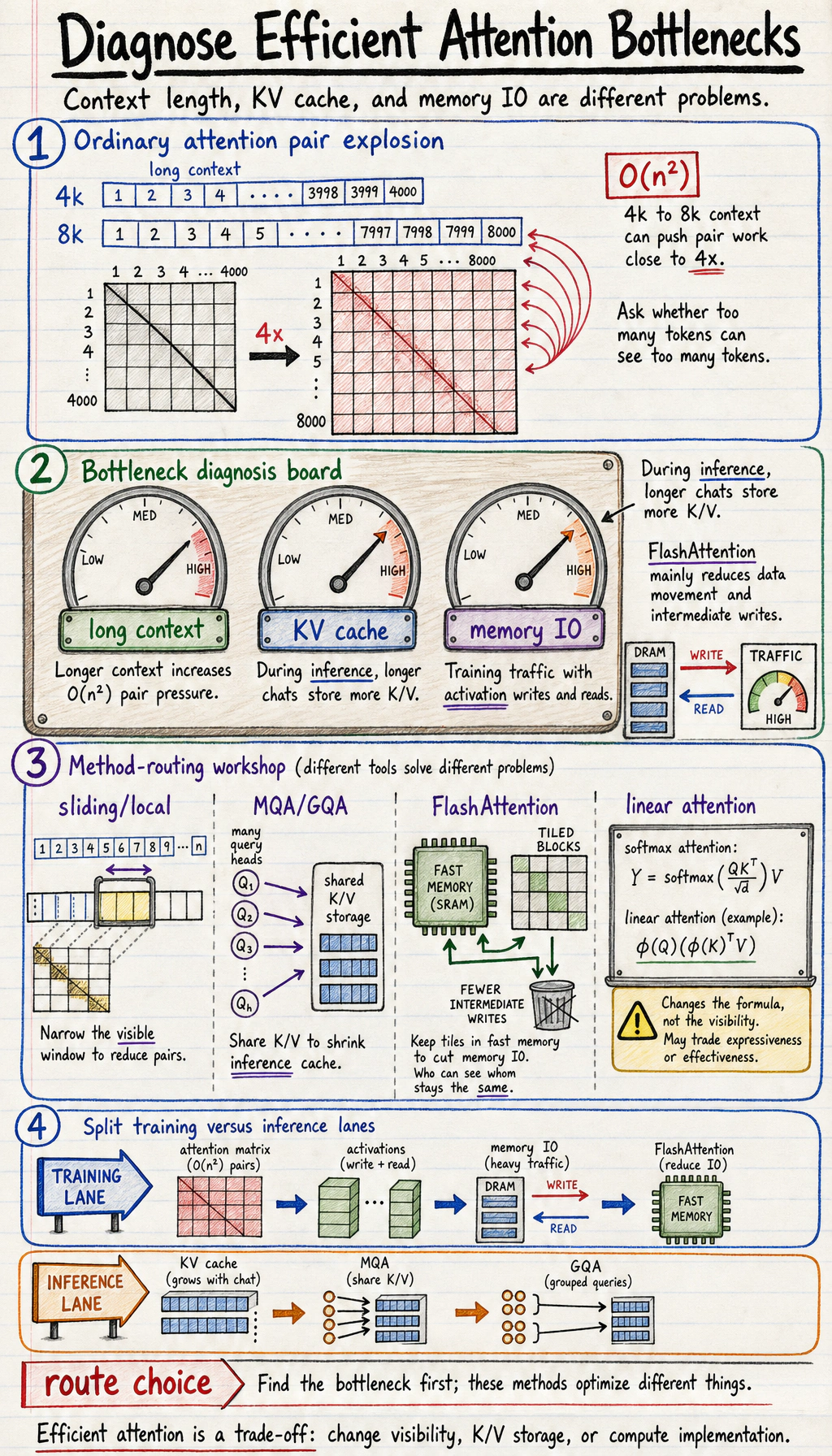
the cost does not simply multiply by 2. Many parts are close to multiplying by 4.

So the real challenge of long-context models is not the phrase “support more tokens,” but rather:

How do we support more tokens without letting the cost explode?

Training and inference do not suffer in exactly the same way

During training, the more common pressure comes from:

• Attention matrices being too large
• Too many intermediate activations

During inference, the more common pressure comes from:

• KV cache growing larger and larger
• Longer conversations becoming slower and more memory-hungry

So efficient attention methods also follow different paths. They are not all solving the same problem.

---

First separate the main approaches

Sliding window / local attention: reduce “who looks at whom”

The most intuitive approach is:

• Do not let every token look at the whole world
• Only let it look at a small nearby window

This is like saying:

• Far-away information is not completely useless
• But not every layer and every position needs full alignment

Typical ideas include:

• sliding window attention
• local attention

MQA / GQA: reduce KV cache size

Another very important approach does not change the mask, but changes how K / V are organized in multi-head attention.

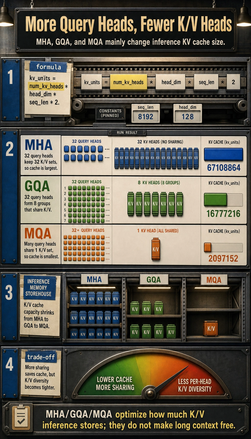
In ordinary multi-head attention, different heads often have their own K/V sets. This makes the inference-time KV cache very large.

So we get:

• MQA: multiple query heads share one set of K/V
• GQA: query heads are grouped and share K/V within each group

Their core benefit is more about:

• lower inference memory usage
• better throughput

FlashAttention: not changing the formula, but changing how it is computed

FlashAttention is often misunderstood as:

• a new definition of attention

A more accurate understanding is:

The attention formula basically stays the same, but more efficient block-wise computation and memory access reduce GPU memory usage and memory traffic waste.

Its main optimization target is:

• implementation efficiency during training and inference

It is not about making the model suddenly understand completely different relationships.

Reading guide

You do not need to memorize the method names in this figure. First separate the bottlenecks: when the context is too long, look at sliding/local attention; when the KV cache is too large, look at MQA/GQA; when memory reads and writes are too expensive, look at FlashAttention. Efficient attention is a set of engineering trade-offs, not a universal formula.

Linear attention: trying to reduce complexity at the formula level

There is also a more aggressive class of methods. It directly rewrites the attention computation and hopes to reduce complexity from quadratic to something lower.

These methods usually trade off among:

• theoretical complexity
• expressive power
• actual effectiveness

---

First run a real example that shows the point

The example below compares two things:

1. Global attention: every position can see all positions
2. Local attention: every position can only see a nearby window

We will not only compare “who can be seen,” but also compare the number of pairs that need to be processed.

from math import exp

values = [0.2, 0.1, 0.0, 0.8, 0.9, 0.7, 0.1, 0.0]


def softmax(scores):
    m = max(scores)
    exps = [exp(x - m) for x in scores]
    total = sum(exps)
    return [x / total for x in exps]


def attention_outputs(sequence, window=None):
    outputs = []
    pairs = 0
    neighborhoods = []

    for i in range(len(sequence)):
        if window is None:
            neighbors = list(range(len(sequence)))
        else:
            left = max(0, i - window)
            right = min(len(sequence), i + window + 1)
            neighbors = list(range(left, right))

        neighborhoods.append(neighbors)
        pairs += len(neighbors)

        scores = [sequence[i] * sequence[j] for j in neighbors]
        weights = softmax(scores)
        output = sum(w * sequence[j] for w, j in zip(weights, neighbors))
        outputs.append(output)

    return outputs, pairs, neighborhoods


full_outputs, full_pairs, full_neighbors = attention_outputs(values, window=None)
local_outputs, local_pairs, local_neighbors = attention_outputs(values, window=2)

print("full pairs :", full_pairs)
print("local pairs:", local_pairs)
print("token 4 full neighbors :", full_neighbors[4])
print("token 4 local neighbors:", local_neighbors[4])
print("full outputs :", [round(x, 3) for x in full_outputs])
print("local outputs:", [round(x, 3) for x in local_outputs])

Expected output:

full pairs : 64
local pairs: 34
token 4 full neighbors : [0, 1, 2, 3, 4, 5, 6, 7]
token 4 local neighbors: [2, 3, 4, 5, 6]
full outputs : [0.376, 0.363, 0.35, 0.457, 0.47, 0.443, 0.363, 0.35]
local outputs: [0.101, 0.285, 0.4, 0.604, 0.615, 0.592, 0.44, 0.267]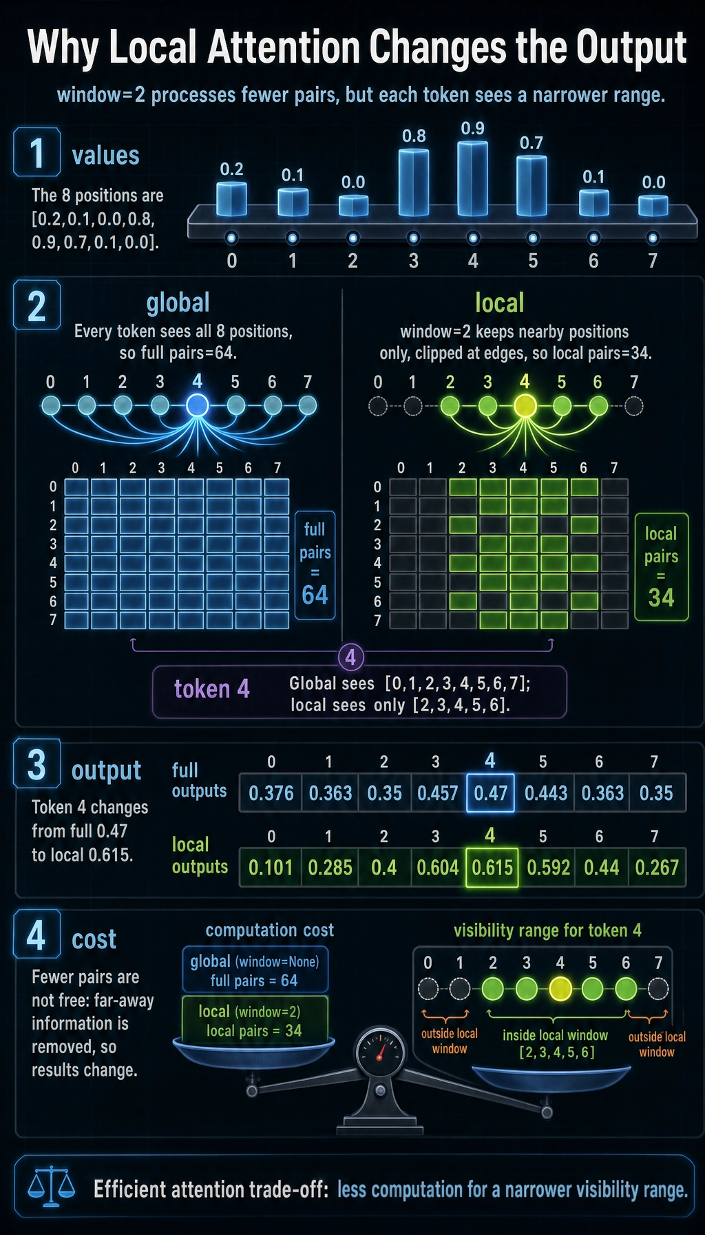

What intuition does this code actually represent?

It tells you two especially important things:

1. If each position is limited to local attention, the number of pairs drops significantly
2. But the output also changes, because the model loses far-away information

This is the core reality of efficient attention:

You are not getting speedup for free; you are trading off efficiency against visibility range.

Why are full pairs and local pairs so different?

Because in global attention, each position looks at every position. In local attention, each position only looks at its nearby window.

When the sequence becomes very long, this gap grows quickly.

Why is local attention not necessarily worse?

Because a lot of information is inherently local. For example, in language:

• The most recent few tokens are often the most relevant
• Long-range dependencies matter, but not every layer needs to model them fully

That is why many long-context models use:

• some global layers
• some local layers
• or mixed schemes with sparse patterns

---

Another major inference-time cost: KV cache

Why does a longer chat use more memory during inference?

Because in decoder-only models, the K / V from each previous step are cached for reuse by later tokens.

This is the:

• KV cache

It significantly reduces repeated computation, but the trade-off is:

• the longer the conversation, the larger the cache

What exactly do MQA / GQA save?

They do not save the attention matrix itself, but rather the amount of K/V that needs to be stored at each layer and each step.

In simple terms:

• Ordinary MHA: each head has its own K/V
• MQA: many query heads share one set of K/V
• GQA: a group of query heads shares one set of K/V

So they are especially suitable for:

• large-model inference
• long conversations
• high-throughput serving

A simple estimate of “which one is cheaper”

def kv_units(num_query_heads, num_kv_heads, head_dim, seq_len):
    return num_kv_heads * head_dim * seq_len * 2


seq_len = 8192
head_dim = 128

print("MHA units =", kv_units(32, 32, head_dim, seq_len))
print("GQA units =", kv_units(32, 8, head_dim, seq_len))
print("MQA units =", kv_units(32, 1, head_dim, seq_len))

Expected output:

MHA units = 67108864
GQA units = 16777216
MQA units = 2097152

These numbers are not a complete GPU memory formula, but they are enough to build an initial intuition:

• the fewer num_kv_heads there are
• the smaller the KV cache becomes

Reading guide

This figure is best understood from an inference perspective: in ordinary MHA, each query head often has its own K/V; GQA makes a group of query heads share K/V; MQA makes even more heads share the same K/V. The more sharing there is, the smaller the KV cache becomes, but you also need to accept some trade-off in expressive power.

---

Why is FlashAttention mentioned so often?

Because many bottlenecks are not about “can’t compute,” but about “moving data is too expensive”

A common issue in attention implementations is:

• intermediate matrices are too large
• GPU memory reads and writes are frequent

The key idea behind FlashAttention is:

• compute in blocks
• minimize writing intermediate results back to expensive memory

So it often brings:

• higher throughput
• lower memory usage

It is not the same kind of thing as sliding window

This point is very important.

• Sliding window changes “who can see whom”
• FlashAttention changes “how it is computed”

So they can even be combined. They are not mutually exclusive.

---

When should you think about which route first?

If your main bottleneck is training memory for long contexts

You will first think of:

• FlashAttention
• activation checkpointing
• sequence parallelism

If your main bottleneck is a too-large KV cache during inference

You will first think of:

• MQA
• GQA
• KV cache quantization

If your main bottleneck is the quadratic complexity of ultra-long contexts

You will first think of:

• sliding window
• sparse attention
• block-wise or hybrid attention
• linear attention-like methods

In other words:

Efficient attention is not one hammer, but a set of tools for different bottlenecks.

---

Common misconceptions

Misconception 1: Efficient attention = faster and definitely better

Many methods are essentially trading off:

• speed
• memory
• receptive field
• implementation complexity

You cannot get all metrics for free.

Misconception 2: As long as a model supports long context, it must be able to “use” long context

Supporting a 128k context does not mean the model can truly and stably use the key information in those 128k tokens.

These are two different things:

• engineering support for length
• the model’s effective use of length

Misconception 3: FlashAttention is a new model architecture

It is not. It is more like an efficient implementation technique.

---

Evidence to Keep

Keep this page’s proof of learning as a small evidence card:

Cost Source

ordinary attention stores or computes seq_len x seq_len interactions

Approach

sparse, linear, FlashAttention, or KV cache depending on bottleneck

Kv Cache

speeds decoding but consumes memory

Hardware Note

algorithm benefit depends on runtime/kernel support

Decision

measure latency/memory before changing architecture

Summary

The most important thing in this section is not memorizing a list of method names, but first separating the problem:

Are you being limited by quadratic complexity, by the KV cache, or by memory read/write efficiency?

Only after identifying the bottleneck do you know which kind of solution to look at:

• sliding window
• GQA / MQA
• FlashAttention

---

Exercises

1. Change window=2 in the example to window=1 or window=3 and observe how the pair count changes.
2. Explain in your own words: why is sliding window changing “who can see whom,” while FlashAttention is changing “how it is computed”?
3. If you are building a long-conversation inference service, why do GQA / MQA often come into view before sliding window?
4. Think about it: why are supporting very long contexts and truly being able to use them effectively not the same thing?

Reference implementation and walkthrough

1. A smaller window reduces the number of visible pairs; a larger window increases it. The exact count should grow with the amount of local context each token is allowed to see.
2. Sliding window changes the attention pattern by limiting visible neighbors. FlashAttention keeps the mathematical attention result but computes it with a more memory-efficient kernel.
3. Long-conversation services often hit KV cache memory first. GQA / MQA reduce the key-value cache footprint, so they can improve serving capacity even when the attention pattern stays full.
4. A model may accept many tokens but still fail to retrieve, connect, or prioritize the right evidence. Context length is a capacity limit; long-context reasoning quality is a behavior that must be evaluated.