3.3.7 Grouping and Aggregation

Pandas GroupBy grouping and aggregation flowchart

Learning objectives

Understand the “split-apply-combine” mechanism of groupby
Master common aggregation functions and the agg method
Learn group-wise transformation (transform) and group-wise filtering (filter)
Master pivot tables (pivot_table)

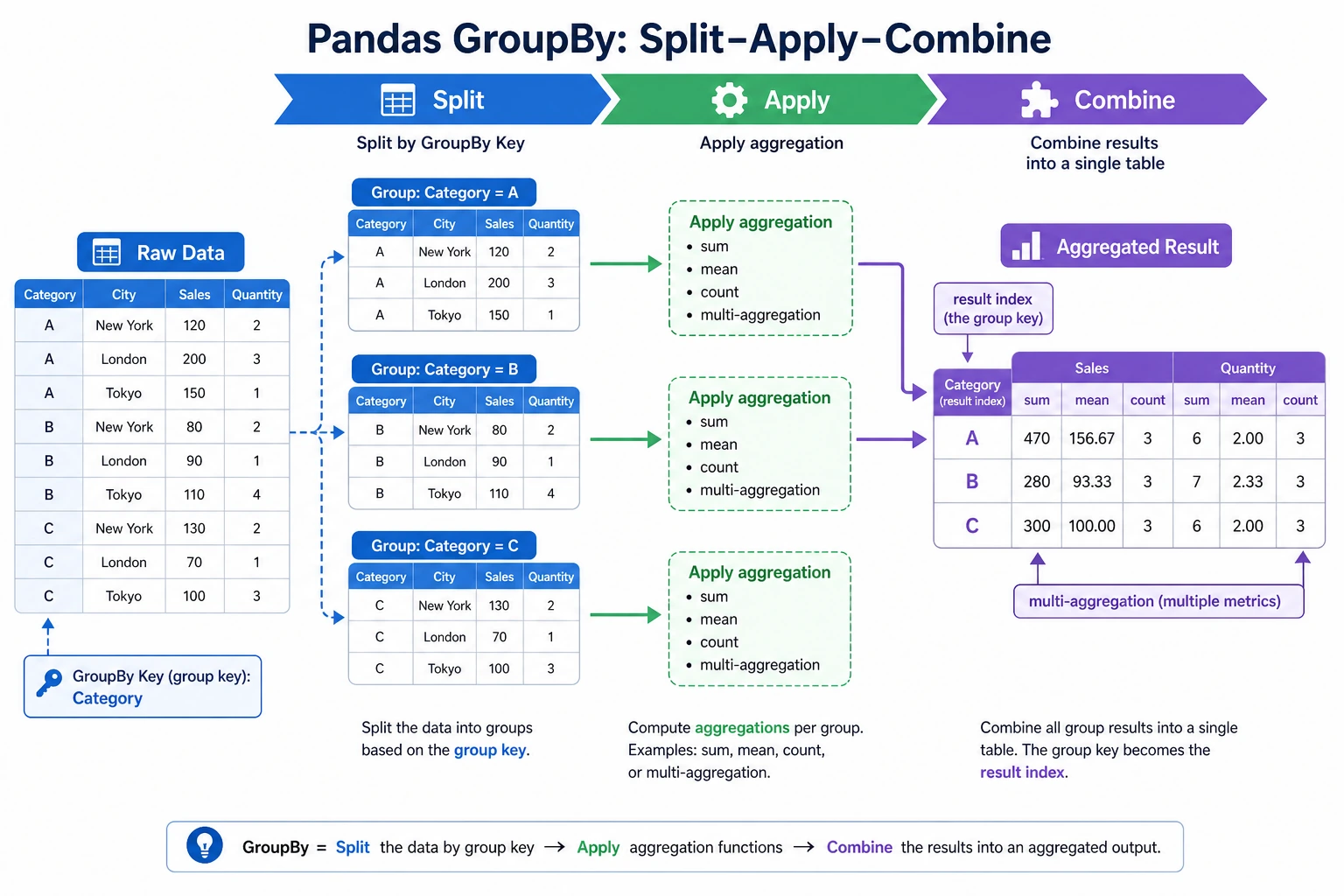
First build a mental map

groupby is easier to understand as “split -> apply -> combine”:

flowchart LR
    A["Raw table"] --> B["Split into multiple groups by a field"]
    B --> C["Perform statistics separately for each group"]
    C --> D["Combine the results again"]

So what this section is really trying to solve is:

Why groupby can handle so many problems like “by department / by category / by month”
What agg / transform / filter / pivot_table each actually adds

Why is groupby so important?

Think back to Chapter 1 — when using pure Python to calculate the survival rate by sex, you had to write dictionaries and loops by hand. With Pandas groupby, you can do it in one line:

# Pure Python: 15 lines of code
# Pandas: 1 line
df.groupby("Sex")["Survived"].mean()

groupby is like SQL GROUP BY — group by a field, then calculate separately for each group.

A more beginner-friendly overall analogy

You can think of groupby as:

First split similar things into piles, then count, calculate, and compare each pile separately

For example:

Group by department
Group by city
Group by month

This is much easier than keeping “Pandas syntax” in your head all the time, and it helps you grasp the essence.

groupby basics

Grouping mechanism

flowchart LR
    A["Raw data"] --> B["Split"]
    B --> C1["Group 1"]
    B --> C2["Group 2"]
    B --> C3["Group 3"]
    C1 --> D["Apply"]
    C2 --> D
    C3 --> D
    D --> E["Combine"]
    E --> F["Result"]

import pandas as pd
import numpy as np

df = pd.DataFrame({
    "Department": ["Engineering", "Marketing", "Engineering", "Management", "Marketing", "Engineering", "Management"],
    "Name": ["Zhang San", "Li Si", "Wang Wu", "Zhao Liu", "Qian Qi", "Sun Ba", "Zhou Jiu"],
    "Salary": [15000, 18000, 22000, 35000, 20000, 19000, 30000],
    "Age": [22, 28, 25, 35, 30, 24, 40]
})

# Group by department and calculate average salary
result = df.groupby("Department")["Salary"].mean()
print(result)
# Department
# Marketing    19000.0
# Engineering  18666.7
# Management   32500.0

Basic aggregation

grouped = df.groupby("Department")

# Common aggregation functions
print(grouped["Salary"].sum())       # Total salary
print(grouped["Salary"].mean())      # Average salary
print(grouped["Salary"].median())    # Median
print(grouped["Salary"].min())       # Lowest salary
print(grouped["Salary"].max())       # Highest salary
print(grouped["Salary"].std())       # Standard deviation
print(grouped["Salary"].count())     # Headcount

Aggregating multiple columns

# Aggregate multiple columns
print(df.groupby("Department")[["Salary", "Age"]].mean())
#                Salary       Age
# Department
# Marketing    19000.0  29.000000
# Engineering  18666.7  23.666667
# Management   32500.0  37.500000

Multi-level grouping

df2 = pd.DataFrame({
    "Department": ["Engineering", "Engineering", "Marketing", "Marketing", "Engineering", "Marketing"],
    "Level": ["Junior", "Senior", "Junior", "Senior", "Junior", "Junior"],
    "Salary": [15000, 25000, 12000, 22000, 18000, 14000]
})

# Group by department and level
result = df2.groupby(["Department", "Level"])["Salary"].mean()
print(result)
# Department  Level
# Marketing   Junior    13000.0
#             Senior    22000.0
# Engineering Junior    16500.0
#             Senior    25000.0

The safest default order when you solve grouping problems for the first time

A safer order is usually:

First ask yourself what to group by
Then ask what to calculate for each group
Finally decide whether you want a summary table or whether you need to write the result back to the original table

This step is very important because it directly determines whether you should use:

agg
transform
filter

`agg`: do multiple aggregations at once

agg lets you apply different aggregation functions to the same column or different columns:

# Calculate multiple statistics for the salary column at once
result = df.groupby("Department")["Salary"].agg(["mean", "min", "max", "count"])
print(result)
#            mean    min    max  count
# Department
# Marketing  19000.0  18000  20000      2
# Engineering 18666.7  15000  22000      3
# Management  32500.0  30000  35000      2

# Use different aggregation functions for different columns
result = df.groupby("Department").agg({
    "Salary": ["mean", "max"],
    "Age": ["mean", "min"],
    "Name": "count"           # Headcount
})
print(result)

# Custom aggregation function
result = df.groupby("Department")["Salary"].agg(
    AverageSalary="mean",
    HighestSalary="max",
    SalaryGap=lambda x: x.max() - x.min()
)
print(result)

When should you think of `agg` first?

When your question sounds like:

“What are the average, maximum, and count for each department?”

At that point, you should usually think first of:

groupby(...).agg(...)

In other words, agg is best for:

Doing multiple summary statistics in one go

`transform`: group-wise transformation

transform applies a function to each group, but it returns a result with the same length as the original data — perfect for creating new columns.

# Scenario: label each person with "difference from department average salary"
df["DepartmentMeanSalary"] = df.groupby("Department")["Salary"].transform("mean")
df["SalaryGap"] = df["Salary"] - df["DepartmentMeanSalary"]
print(df[["Name", "Department", "Salary", "DepartmentMeanSalary", "SalaryGap"]])

# Scenario: within-group standardization (subtract mean and divide by std for each group)
df["Salary_Standardized"] = df.groupby("Department")["Salary"].transform(
    lambda x: (x - x.mean()) / x.std() if x.std() > 0 else 0
)

The difference between transform and agg

agg: returns one value per group (summary), so the number of rows equals the number of groups
transform: returns the same number of values as the original data, so the number of rows equals the original number of rows

# agg: 3 departments → 3 rows
df.groupby("Department")["Salary"].agg("mean")

# transform: 7 people → 7 rows (each person gets their department mean)
df.groupby("Department")["Salary"].transform("mean")

A comparison table that is very useful for beginners to remember first

Method	Return shape
`agg`	One summary result per group
`transform`	Same number of rows, just add a “group statistic” column
`filter`	Keep or remove entire groups
`pivot_table`	Organize results into a cross table

This table is especially useful for beginners because it helps separate several easily confused methods again.

`filter`: group-wise filtering

filter keeps or removes whole groups based on a condition:

# Keep only departments with average salary > 20000
result = df.groupby("Department").filter(lambda x: x["Salary"].mean() > 20000)
print(result)
# Only the "Management" department has an average salary > 20000, so only people in Management are kept

# Keep only departments with at least 3 people
result = df.groupby("Department").filter(lambda x: len(x) >= 3)
print(result)

Pivot tables (`pivot_table`)

Pivot tables are a very familiar feature for Excel users — and Pandas supports them perfectly.

# Prepare sales data
sales = pd.DataFrame({
    "Month": ["Jan", "Jan", "Feb", "Feb", "Jan", "Feb"],
    "Product": ["Apple", "Milk", "Apple", "Milk", "Bread", "Bread"],
    "SalesVolume": [50, 30, 60, 25, 40, 45],
    "Amount": [250, 240, 300, 200, 120, 135]
})

# Pivot table: total sales volume of each product by month
pivot = pd.pivot_table(
    sales,
    values="SalesVolume",        # Value to aggregate
    index="Product",             # Rows
    columns="Month",             # Columns
    aggfunc="sum"                # Aggregation method
)
print(pivot)
# Month   Jan   Feb
# Product
# Milk     30   25
# Apple    50   60
# Bread    40   45

# Multiple aggregations
pivot2 = pd.pivot_table(
    sales,
    values="Amount",
    index="Product",
    columns="Month",
    aggfunc=["sum", "mean"],
    margins=True              # Add total rows and columns
)
print(pivot2)

Crosstab

# Count the distribution of people across departments and levels
ct = pd.crosstab(df2["Department"], df2["Level"])
print(ct)
# Level  Junior  Senior
# Department
# Marketing    2    1
# Engineering  2    1

# Add totals and proportions
ct2 = pd.crosstab(df2["Department"], df2["Level"], margins=True, normalize="index")
print(ct2)  # Row-wise proportions (the share of Junior/Senior within each department)

Practice: sales data grouping analysis

import pandas as pd
import numpy as np

rng = np.random.default_rng(seed=42)
n = 200

orders = pd.DataFrame({
    "Month": rng.choice(["Jan", "Feb", "Mar", "Apr"], n),
    "Region": rng.choice(["East China", "South China", "North China", "Southwest"], n),
    "Product": rng.choice(["Phone", "Computer", "Headphones", "Tablet"], n),
    "SalesVolume": rng.integers(1, 50, n),
    "UnitPrice": rng.choice([99, 299, 999, 2999, 5999], n)
})
orders["Amount"] = orders["SalesVolume"] * orders["UnitPrice"]

# 1. Total sales amount for each region
print(orders.groupby("Region")["Amount"].sum().sort_values(ascending=False))

# 2. Average sales volume and total amount for each product
print(orders.groupby("Product").agg(
    AverageSalesVolume=("SalesVolume", "mean"),
    TotalAmount=("Amount", "sum"),
    OrderCount=("Amount", "count")
))

# 3. Pivot table: total amount by region × product
print(pd.pivot_table(orders, values="Amount", index="Region", columns="Product", aggfunc="sum"))

# 4. The region with the highest sales amount in each month
monthly_top = orders.groupby(["Month", "Region"])["Amount"].sum().reset_index()
idx = monthly_top.groupby("Month")["Amount"].idxmax()
print(monthly_top.loc[idx])

Evidence to Keep

Keep this page’s proof of learning as a small evidence card:

Dataframe State: columns, dtypes, row count, missing values, and sample rows
Operation: read/write, select/filter, clean, transform, groupby, merge, or time-series step
Output: resulting table, saved file, aggregation, join result, or time index view
Failure Check: dtype mismatch, missing data, duplicated keys, chained assignment, or wrong time frequency
Expected Output: before/after table sample with the transformation reason

Summary

Operation	Method	Number of rows returned	Use case
Basic aggregation	`groupby().mean()` etc.	Number of groups	Summary statistics
Multiple aggregations	`groupby().agg()`	Number of groups	Multiple statistics
Group-wise transformation	`groupby().transform()`	Original number of rows	Create new columns
Group-wise filtering	`groupby().filter()`	≤ original number of rows	Keep groups by condition
Pivot table	`pivot_table()`	Number of unique row values	Cross-tabulation
Crosstab	`crosstab()`	Number of unique row values	Frequency statistics

Hands-on exercises

Exercise 1: basic grouping

# Use the orders data above
# 1. Calculate the average order value by month (amount / volume)
# 2. Which month and product had the highest sales volume?
# 3. Which product sold best in each region?

Exercise 2: `transform` practice

# 1. Add a "region average amount" column to each order
# 2. Mark whether each order amount is above the average of its region
# 3. Calculate what percentage each order amount contributes to the total amount of its region

Exercise 3: pivot tables

# 1. Create a pivot table: rows = region, columns = month, values = total amount, with totals
# 2. In which month did each region have the highest sales amount?

Reference implementation and walkthrough

Average order value is total amount divided by order count, so compute both numerator and denominator instead of averaging already-averaged rows.
For best product by month or region, aggregate to the correct level first, then sort or use idxmax. Picking the maximum raw row can give the wrong answer when a product appears many times.
Use transform when each original row needs a group-level value, such as region average or share of monthly sales. Use agg when the output should be one row per group.