5.1.2 What Is Machine Learning

Where This Section Fits

This is your first stop as you officially enter machine learning. The key is not memorizing definitions, but understanding the difference between machine learning and traditional programming, and building a framework for deciding “problem type → data format → learning method.” This will lay the foundation for supervised learning, unsupervised learning, and model evaluation later on.

Welcome to the Machine Learning Stage

In the first three stages, you learned Python, data analysis, and math fundamentals. Now, you’re finally going to let the computer learn things by itself. This is one of the most exciting stages in the entire AI journey.

Learning Objectives

• Understand what machine learning is and how it differs from traditional programming
• Master the three major categories of machine learning (supervised learning, unsupervised learning, reinforcement learning)
• Understand the complete machine learning workflow
• Build the right ML thinking framework

---

First, Build a Map

The most important task in this article is not memorizing the definition, but first building a decision framework:

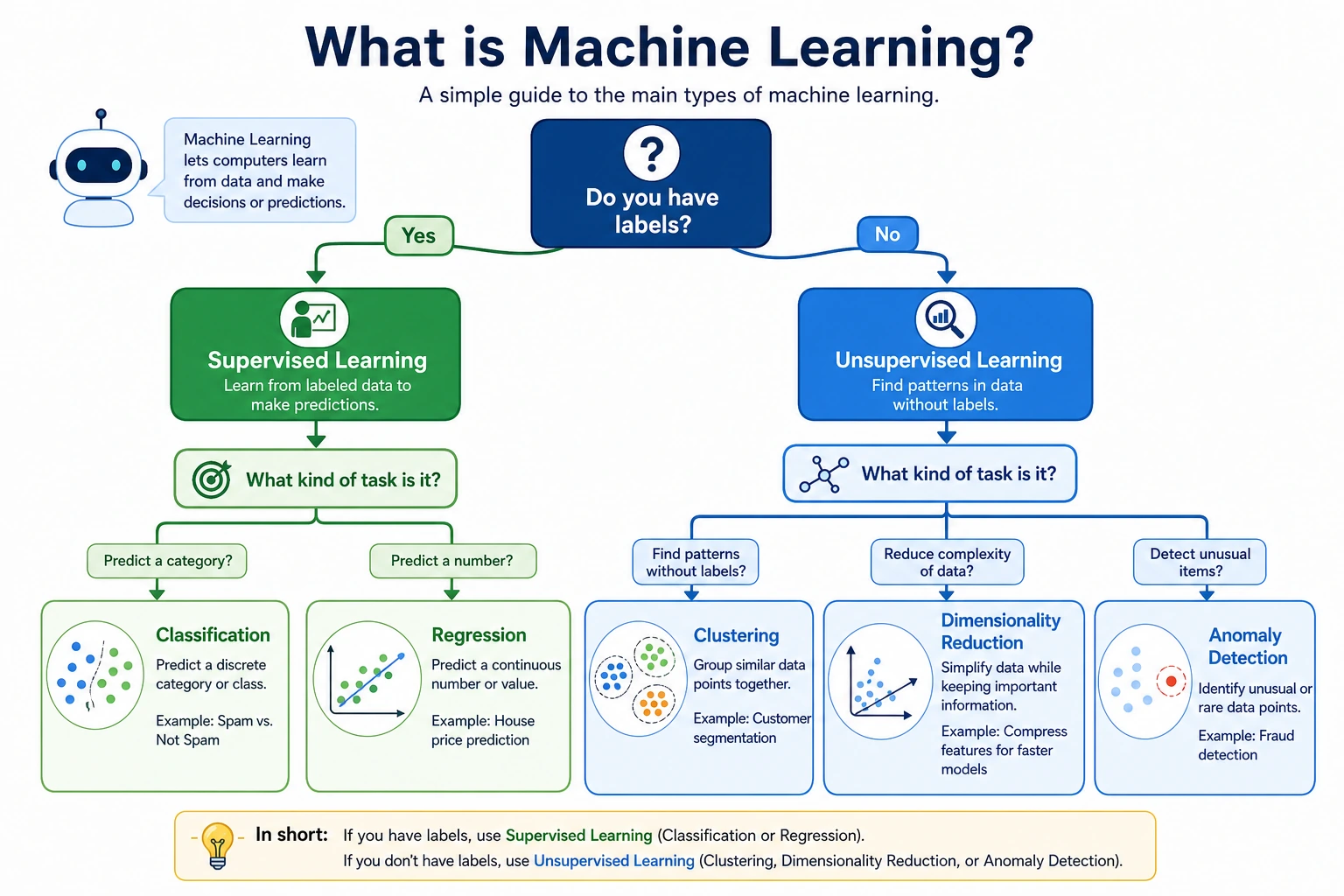
If you understand this diagram, many chapters later in Stage 5 will suddenly start making sense.

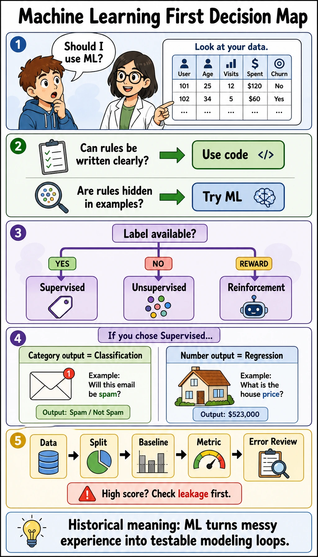
Use this comic as a quick entry checklist: if rules can be written clearly, normal programming may be enough; if the rule is hidden in many examples, machine learning becomes useful. Then decide whether you have labels, whether the output is a category or a number, and whether the evaluation metric can prove the model is useful.

---

What Exactly Is Machine Learning?

One-Sentence Definition

Machine learning = letting a computer automatically discover patterns from data instead of having humans hand-code rules.

Traditional Programming vs. Machine Learning

flowchart LR
    subgraph Traditional Programming
        R1["Humans write rules"] --> P1["Program"]
        D1["Data"] --> P1
        P1 --> O1["Output"]
    end

    subgraph Machine Learning
        D2["Data"] --> ML["Machine learning algorithm"]
        O2["Expected output"] --> ML
        ML --> R2["Automatically learned rules (model)"]
    end

    style R1 fill:#fff3e0,stroke:#e65100,color:#333
    style R2 fill:#e8f5e9,stroke:#2e7d32,color:#333

	Traditional Programming	Machine Learning
Input	Rules + data	Data + expected output
Output	Result	Rules (model)
Suitable for	Clear rules (such as calculating taxes)	Rules that are hard to describe (such as recognizing cats)
How it is built	Humans write if-else logic	Algorithms learn automatically from data

Why Do We Need Machine Learning?

For some tasks, humans cannot clearly describe the rules:

# Traditional programming: determine whether an email is spam
def is_spam_traditional(email):
    if "free" in email:
        return True
    if "winner" in email:
        return True
    if "click to claim" in email:
        return True
    # ... how many more rules are there? You can never finish writing them!
    return False

# Machine learning: give the model 100,000 labeled emails and let it learn by itself
# model.fit(emails, labels)
# model.predict(new_email)  → make an automatic decision

Machine learning is suitable for scenarios such as:

• Complex or unknown rules (image recognition, speech recognition)
• Rules that change over time (recommendation systems, fraud detection)
• Very large datasets that humans cannot analyze manually
• Situations where personalized results are needed

When Learning Machine Learning for the First Time, What Should You Focus on Most?

The first thing to grasp is not “how many kinds of models there are,” but this sentence:

Machine learning replaces hand-written rules with data.

Once you understand that, many questions become easier to judge:

• When traditional programming is suitable
• When to let a model learn
• Why data quality directly determines the upper limit of a model’s performance

Terms Beginners Should Decode Early

Term	What it is	Why it matters in this chapter
ML	Short for Machine Learning	You will see it in diagrams, filenames, and project notes
model	The learned rule or function	It is the thing produced by training and reused for prediction
algorithm	The learning method	A decision tree, logistic regression, or K-Means is an algorithm before training
training	The process of learning from data	In code, this usually happens when you call fit
inference	Using a trained model on new data	In sklearn, this usually appears as predict or predict_proba
baseline	The simplest first result to beat	It tells you whether later improvements are real or just noise
metric	The measurement rule for success	Accuracy, F1, MAE, and RMSE answer different evaluation questions

For beginners, the most important distinction is algorithm vs. model: the algorithm is the learning recipe, while the model is the trained result after the recipe has seen data.

---

The Three Major Categories of Machine Learning

flowchart TD
    ML["Machine Learning"]
    ML --> SL["Supervised Learning"]
    ML --> UL["Unsupervised Learning"]
    ML --> RL["Reinforcement Learning"]

    SL --> CL["Classification<br/>(email → spam/normal)"]
    SL --> RG["Regression<br/>(features → house price prediction)"]

    UL --> CLU["Clustering<br/>(customer segmentation)"]
    UL --> DR["Dimensionality reduction<br/>(data compression)"]

    RL --> G["Game AI"]
    RL --> RO["Robot control"]

    style SL fill:#e3f2fd,stroke:#1565c0,color:#333
    style UL fill:#fff3e0,stroke:#e65100,color:#333
    style RL fill:#e8f5e9,stroke:#2e7d32,color:#333

Supervised Learning — With a “Correct Answer”

Core idea: Give the model lots of input-output pairs and let it learn the mapping relationship.

Type	Output	Example
Classification	Discrete categories	Email → spam/normal, image → cat/dog
Regression	Continuous values	Area → house price, features → temperature

# Data format for supervised learning
# X (features/input)      y (label/output)
# [area, rooms, floor]    → house price
# [120,  3,    15]        → 3.5 million
# [80,   2,    8]         → 2.2 million
# [200,  4,    20]        → 5.8 million

Key point: Training data must have labels (correct answers). The model’s goal is to learn to predict y from X.

How Can You Quickly Tell Whether a Problem Is Supervised Learning?

Ask yourself directly:

• Do I have paired data in the form of “input → correct output”?

If yes, it is usually supervised learning. Then ask:

• Is the output a category or a continuous value?

That will naturally split it into:

• Classification
• Regression

Unsupervised Learning — No “Correct Answer”

Core idea: There are only input data, no labels. The model discovers the structure and patterns in the data by itself.

Type	What it does	Example
Clustering	Groups similar data together	Customer segmentation, news categorization
Dimensionality reduction	Reduces the number of features	PCA (learned in Stage 4)
Anomaly detection	Finds abnormal data	Credit card fraud detection

# Data for unsupervised learning: no labels
# X (features)
# [spending amount, purchase frequency, recent purchase]
# [500,             10,               3 days ago]
# [50,              2,                30 days ago]
# [1000,            20,               1 day ago]
# → The model automatically splits them into groups like "high-value customers" and "low-frequency customers"

The Most Easily Misunderstood Part of Unsupervised Learning

Many beginners think unsupervised learning means “the machine can find the true answer by itself.” A more accurate way to say it is:

• The model helps you discover a possible structure
• But whether that structure has business value still depends on your interpretation

So in unsupervised learning, “explaining the result” is often just as important as “getting the result.”

Reinforcement Learning — Learning Through Trial and Error

Core idea: An agent takes actions in an environment and adjusts its strategy based on rewards and penalties.

Element	Explanation
Agent	The AI making decisions
Environment	The world the agent lives in
State	Information about the current environment
Action	A choice the agent can make
Reward	Feedback received after an action

# Intuition for reinforcement learning: training a puppy
# State: the environment the puppy sees
# Action: sit / stand / shake hands
# Reward: does it correctly → give a treat (+1), does it incorrectly → no treat (0)
# After repeated trial and error, the puppy learns the right behavior

Focus of This Course

At this stage, we mainly learn supervised learning and unsupervised learning. Reinforcement learning will appear later in the agent systems section.

Comparison of the Three Learning Types

	Supervised Learning	Unsupervised Learning	Reinforcement Learning
Labeled data?	Yes	No	Reward signal
Goal	Predict labels	Discover structure	Maximize reward
Typical algorithms	Linear regression, decision trees	K-Means, PCA	Q-Learning, PPO
AI applications	Image classification, translation	Customer segmentation, recommendation	Game AI, robots

---

The Machine Learning Workflow

Complete Workflow

flowchart TD
    A["1. Problem definition<br/>What problem are we solving?"] --> B["2. Data collection<br/>Gather relevant data"]
    B --> C["3. Data preprocessing<br/>Cleaning, feature engineering"]
    C --> D["4. Choose a model<br/>Linear regression? Decision tree?"]
    D --> E["5. Train the model<br/>Fit using training data"]
    E --> F["6. Evaluate the model<br/>Validate using test data"]
    F --> G{"Is the result good?"}
    G -->|"Not good enough"| H["7. Tuning<br/>Adjust parameters, switch models"]
    H --> D
    G -->|"Good enough"| I["8. Deploy to production<br/>Use for real predictions"]

    style A fill:#e3f2fd,stroke:#1565c0,color:#333
    style E fill:#fff3e0,stroke:#e65100,color:#333
    style I fill:#e8f5e9,stroke:#2e7d32,color:#333

Read the Workflow as Plain English First

This workflow can be translated into a simpler sentence for beginners:

First define the problem, then prepare the data, build a version that works, check the results, and finally improve it step by step.

This sentence is actually the underlying logic of the entire main line in Stage 5.

Training Set vs. Test Set

This is one of the most important concepts in ML: you cannot evaluate a model using the training data.

import numpy as np

# Simulated dataset
rng = np.random.default_rng(seed=42)
n = 100
X = rng.normal(size=(n, 3))
y = rng.integers(0, 2, n)

# Usually 80% training, 20% testing
from sklearn.model_selection import train_test_split

X_train, X_test, y_train, y_test = train_test_split(
    X, y, test_size=0.2, random_state=42
)

print(f"Training set: {X_train.shape[0]} samples")
print(f"Test set: {X_test.shape[0]} samples")

Expected output:

Training set: 80 samples
Test set: 20 samples

flowchart LR
    D["All data<br/>100 samples"]
    D -->|"80%"| TR["Training set<br/>80 samples<br/>Used to train the model"]
    D -->|"20%"| TE["Test set<br/>20 samples<br/>Used to evaluate the model"]

    style TR fill:#e3f2fd,stroke:#1565c0,color:#333
    style TE fill:#e8f5e9,stroke:#2e7d32,color:#333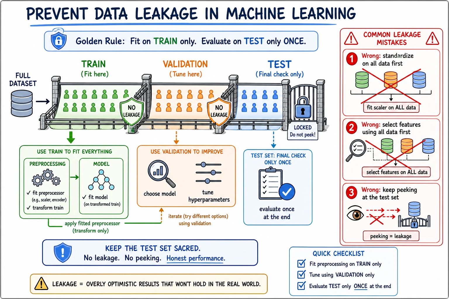

Why Separate Them?

If you train and evaluate on the same data, the model may get a perfect score by “memorizing” the data—but perform poorly on new data. This is called overfitting. It is like memorizing the answers before an exam and then failing when given a different set of questions.

When reading this diagram, first look at the three boundaries: the training set is used for learning, the validation set is used to choose a solution, and the test set is only used for final verification. If any preprocessing step sees test-set information too early—for example, standardizing on the full dataset first or selecting features using the full dataset—the model score may look artificially high.

A Common Beginner Mistake: Confusing “Learning” with “Memorizing”

One especially important boundary in machine learning is:

• Doing well on the training set does not mean the model has truly learned the pattern
• It may just have memorized the training data

So from this section onward, you should build a habit:

• When you see a high score, first ask whether it is a training-set score or a test-set score

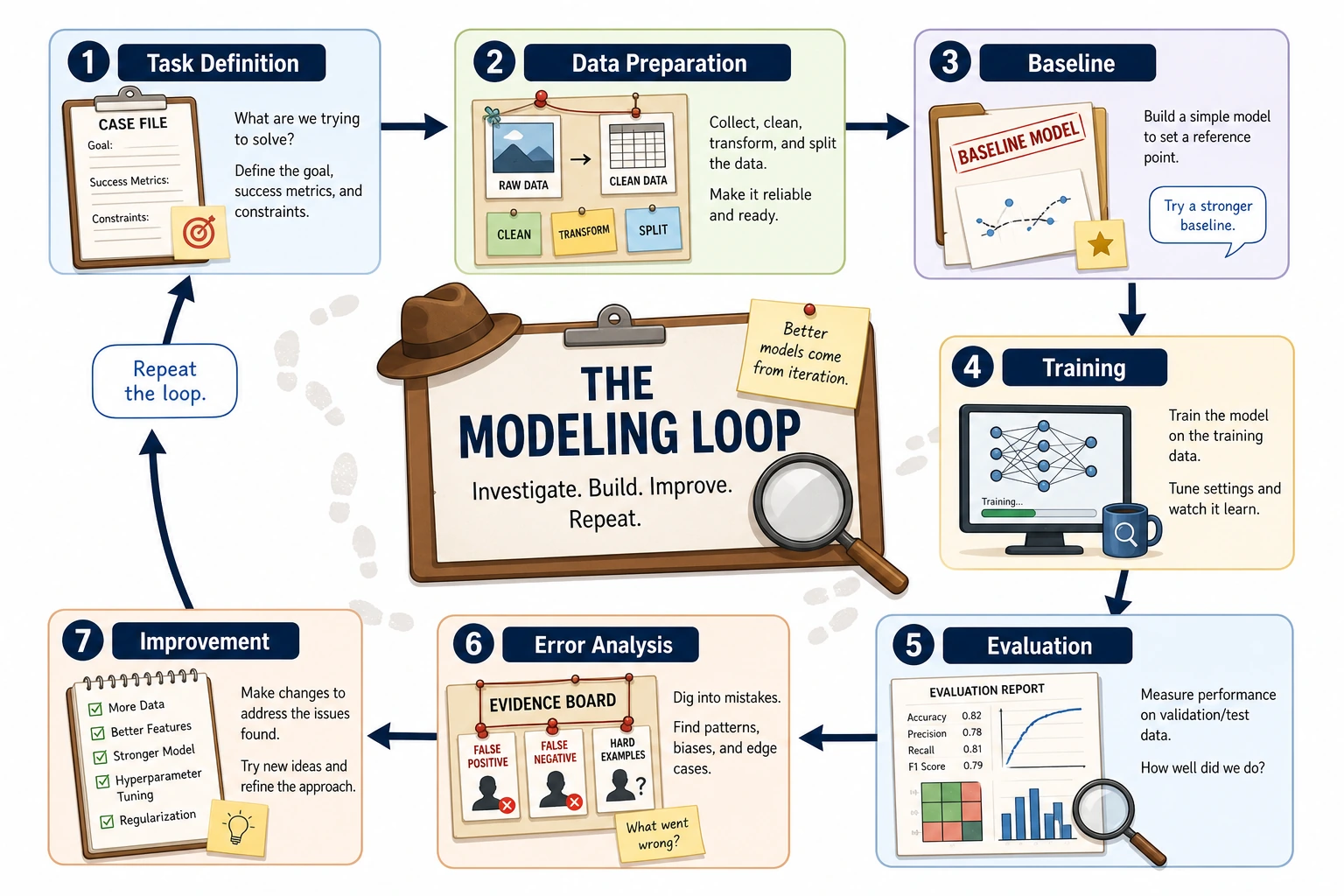
A Minimal Complete Example

Before reading the code, look at the whole loop first:

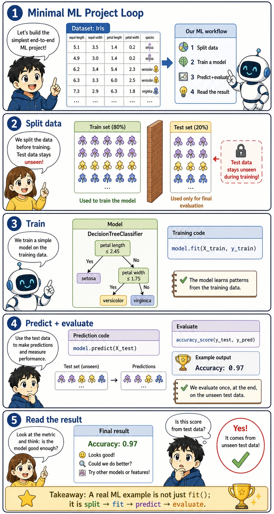
This diagram is the smallest useful ML project shape: define the problem, prepare X and y, train a model, evaluate it with a metric, then decide what to improve. The code below is intentionally tiny so you can connect each line to one step in the picture instead of getting lost in framework details.

from sklearn.datasets import load_iris
from sklearn.model_selection import train_test_split
from sklearn.tree import DecisionTreeClassifier
from sklearn.metrics import accuracy_score

# 1. Load data
iris = load_iris()
X, y = iris.data, iris.target
print(f"Dataset: {X.shape[0]} samples, {X.shape[1]} features, {len(set(y))} classes")

# 2. Split into training and test sets
X_train, X_test, y_train, y_test = train_test_split(X, y, test_size=0.2, random_state=42)

# 3. Choose a model and train it
model = DecisionTreeClassifier(random_state=42)
model.fit(X_train, y_train)  # Train!

# 4. Predict and evaluate
y_pred = model.predict(X_test)
accuracy = accuracy_score(y_test, y_pred)
print(f"Test set accuracy: {accuracy:.1%}")

Expected output:

Dataset: 150 samples, 4 features, 3 classes
Test set accuracy: 100.0%

You can complete a full ML project with just a few lines of code! The next chapters will gradually dive into each part.

If this code fails with ModuleNotFoundError: No module named 'sklearn', install the chapter dependency first:

python -m pip install --upgrade scikit-learn

Here, scikit-learn is the package name you install, while sklearn is the module name you import in Python code.

Read the code with this mapping in mind:

Code keyword	What it means	Why it matters
load_iris()	Loads a built-in toy dataset	It gives us a safe first dataset without downloading files
X	Feature matrix, the input columns	The model learns patterns from these values
y	Target vector, the correct answers	Supervised learning needs labels to learn
train_test_split	Splits data into learning and checking parts	It prevents us from judging the model on examples it already saw
fit	Trains the model	This is where the algorithm becomes a trained model
predict	Uses the trained model on new inputs	This is the inference step used in real applications
accuracy_score	Calculates the percentage of correct predictions	It turns model behavior into a measurable result
random_state	Fixes the random split or model randomness	It makes the example reproducible when learners run it again

---

Key Terms Quick Reference

Term	English	Meaning
Sample	Sample	One data point
Feature	Feature	A property describing the sample (each input column)
Label	Label / Target	The sample’s “answer” (the value to predict)
Training set	Training Set	Data used to train the model
Test set	Test Set	Data used to evaluate the model
Overfitting	Overfitting	The model “memorizes” the training data and generalizes poorly
Underfitting	Underfitting	The model is too simple and cannot even learn the training data well
Generalization	Generalization	The ability of a model to perform well on new data
Hyperparameter	Hyperparameter	A parameter set by humans, such as learning rate or tree depth
Data leakage	Data leakage	Test or future information accidentally enters training, making the score look better than it really is
Validation set	Validation Set	Data used to choose models or hyperparameters before the final test

Overfitting vs. Underfitting

flowchart LR
    A["Underfitting<br/>Model is too simple<br/>Fitting curve data with a straight line"]
    B["Just right<br/>Model complexity is appropriate<br/>Fits the pattern well"]
    C["Overfitting<br/>Model is too complex<br/>Even fits the noise"]

    style A fill:#ffebee,stroke:#c62828,color:#333
    style B fill:#e8f5e9,stroke:#2e7d32,color:#333
    style C fill:#ffebee,stroke:#c62828,color:#333

import matplotlib.pyplot as plt

rng = np.random.default_rng(seed=42)
x = np.linspace(0, 1, 20)
y = np.sin(2 * np.pi * x) + rng.normal(size=20) * 0.3

fig, axes = plt.subplots(1, 3, figsize=(15, 4))
x_smooth = np.linspace(0, 1, 200)

# Underfitting: 1st-degree polynomial (straight line)
coeffs = np.polyfit(x, y, 1)
axes[0].scatter(x, y, color='steelblue', s=40)
axes[0].plot(x_smooth, np.polyval(coeffs, x_smooth), 'r-', linewidth=2)
axes[0].set_title('Underfitting (straight line)\nToo simple to capture the pattern')

# Just right: 3rd-degree polynomial
coeffs = np.polyfit(x, y, 3)
axes[1].scatter(x, y, color='steelblue', s=40)
axes[1].plot(x_smooth, np.polyval(coeffs, x_smooth), 'r-', linewidth=2)
axes[1].set_title('Just right (3rd-degree polynomial)\nFits the pattern well')

# Overfitting: 18th-degree polynomial
coeffs = np.polyfit(x, y, 18)
axes[2].scatter(x, y, color='steelblue', s=40)
y_overfit = np.polyval(coeffs, x_smooth)
y_overfit = np.clip(y_overfit, -3, 3)
axes[2].plot(x_smooth, y_overfit, 'r-', linewidth=2)
axes[2].set_title('Overfitting (18th-degree polynomial)\nEven fits the noise')
axes[2].set_ylim(-3, 3)

for ax in axes:
    ax.grid(True, alpha=0.3)

plt.tight_layout()
plt.show()

---

Evidence to Keep

Keep this page’s proof of learning as a small evidence card:

Ml Problem

supervised, unsupervised, evaluation, or feature-engineering task

Baseline

simplest sklearn/modeling loop and fixed train/test split

Output

prediction, metric, chart, or model decision note

Failure Check

data leakage, unclear target, weak baseline, or metric mismatch

Expected Output

minimal ML loop with metric and one failure observation

Summary

Key point	Explanation
Machine learning	Letting computers learn patterns from data
Supervised learning	Has labels and learns prediction (classification/regression)
Unsupervised learning	No labels and discovers structure (clustering/dimensionality reduction)
Reinforcement learning	Learns strategies through trial and error (reward-driven)
Core workflow	Data → preprocessing → training → evaluation → deployment
Training/test split	Must be separated to prevent overfitting

What Should You Take Away from This Section?

If you only take away one sentence, I hope you remember this:

The real starting point of the machine learning stage is not learning a specific model, but first learning how to match the problem, the data, and the evaluation method.

So the most important gains from this section should be:

• Be able to distinguish supervised learning from unsupervised learning
• Be able to distinguish classification from regression
• Know why training and test sets must be separated
• Know that all the algorithms later in Stage 5 are actually part of this map

Connect to What Comes Next

• Next section: Introduction to the Scikit-learn framework — the standard tool for ML practice
• Chapter 2: Learn specific algorithms (linear regression, logistic regression, decision trees, etc.)
• Chapter 4: Deep dive into model evaluation — how to scientifically judge whether a model is good

---

Hands-On Exercises

Exercise 1: Classification vs. Regression

Determine whether each task is classification or regression:

1. Predict tomorrow’s temperature
2. Determine whether a photo contains a face
3. Predict tomorrow’s closing price of a stock
4. Classify news into sports/technology/entertainment/finance
5. Predict whether a user will churn

Exercise 2: Your First ML Model

Use scikit-learn’s load_wine() dataset to train a decision tree classifier and output the test-set accuracy.

from sklearn.datasets import load_wine
from sklearn.model_selection import train_test_split
from sklearn.tree import DecisionTreeClassifier

wine = load_wine()
X_train, X_test, y_train, y_test = train_test_split(
    wine.data, wine.target, test_size=0.2, random_state=42, stratify=wine.target
)

model = DecisionTreeClassifier(random_state=42)
model.fit(X_train, y_train)
accuracy = model.score(X_test, y_test)
print(f"Test accuracy: {accuracy:.3f}")

Expected output on a current sklearn version:

Test accuracy: 0.944

Your exact result may change slightly if the sklearn version or split settings change. What matters here is the workflow: load data, split data, train on the training set, and evaluate on the test set.

Exercise 3: Observe Overfitting

Modify the overfitting example in section 4.3, use polynomials of different degrees (1, 3, 5, 10, 18) to fit the data, plot 5 subplots, and observe how complexity affects the fitting result.

Reference implementation and walkthrough

1. Temperature and stock closing price are regression tasks because the target is numeric. Face detection, news category, and churn are classification tasks because the target is a discrete class.
2. The wine example should follow the core supervised workflow: load features and labels, split before training, fit only on X_train, y_train, then score on X_test, y_test. A result near 0.944 is plausible for this split, but the exact value is less important than avoiding test-set leakage.
3. Degree 1 usually underfits, degrees 3 or 5 often capture the main pattern, and degrees 10 or 18 can chase noise. Judge complexity with held-out error as well as the plot, because a curve that hugs training points may generalize poorly.