5.2.3 Logistic Regression

Section Positioning

Logistic regression has “regression” in its name, but in practice it is a classification model. It learns a linear score, turns that score into a probability, and then uses a threshold to make a class decision.

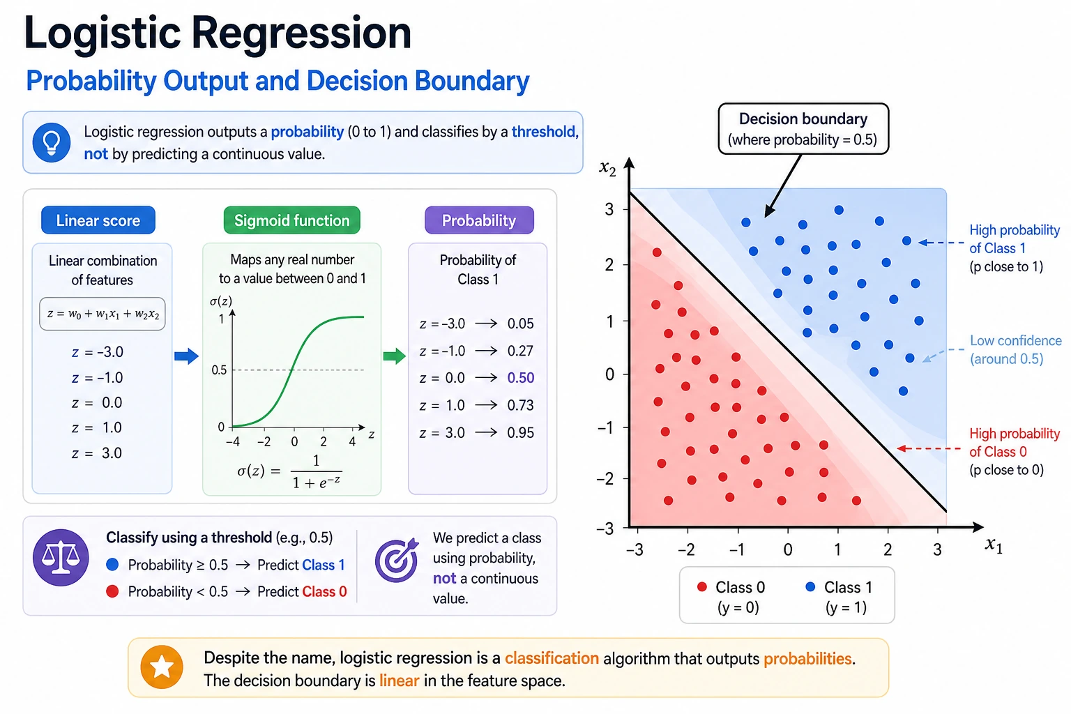
What You Will Build

By the end of this lesson you will have a runnable classification workflow that can:

• train a binary classifier with Pipeline, StandardScaler, and LogisticRegression;
• print accuracy, precision, recall, F1, false positives, and false negatives;
• change the classification threshold instead of blindly using 0.5;
• inspect which standardized features matter most;
• compare regularization strength with C;
• run the same model pattern on a multi-class dataset.

First read the two maps, then run the code. The details below will make much more sense after you see real output.

Setup

Run this in a clean virtual environment:

python -m pip install -U scikit-learn numpy

This lesson uses the current stable scikit-learn API style: Pipeline for safe preprocessing, StandardScaler for numeric feature scaling, and LogisticRegression without deprecated multi-class flags.

Run the Complete Lab

Create logistic_lab.py:

import numpy as np
from sklearn.datasets import load_breast_cancer, load_iris
from sklearn.linear_model import LogisticRegression
from sklearn.metrics import accuracy_score, confusion_matrix, f1_score, precision_score, recall_score
from sklearn.model_selection import train_test_split
from sklearn.pipeline import Pipeline
from sklearn.preprocessing import StandardScaler


def make_model(C=1.0):
    return Pipeline([
        ("scale", StandardScaler()),
        ("clf", LogisticRegression(max_iter=2000, C=C, random_state=42)),
    ])


# Part 1: binary classification and threshold tuning.
cancer = load_breast_cancer()
X_train, X_test, y_train, y_test = train_test_split(
    cancer.data,
    cancer.target,
    test_size=0.25,
    random_state=42,
    stratify=cancer.target,
)

model = make_model(C=1.0)
model.fit(X_train, y_train)
prob = model.predict_proba(X_test)[:, 1]

print("binary_threshold_lab")
for threshold in [0.3, 0.5, 0.7]:
    pred = (prob >= threshold).astype(int)
    tn, fp, fn, tp = confusion_matrix(y_test, pred).ravel()
    print(
        f"threshold={threshold:.1f} "
        f"accuracy={accuracy_score(y_test, pred):.3f} "
        f"precision={precision_score(y_test, pred):.3f} "
        f"recall={recall_score(y_test, pred):.3f} "
        f"f1={f1_score(y_test, pred):.3f} "
        f"fp={fp} fn={fn}"
    )

clf = model.named_steps["clf"]
top = np.abs(clf.coef_[0]).argsort()[-3:][::-1]
print("top_scaled_coefficients")
for idx in top:
    print(f"- {cancer.feature_names[idx]}: {clf.coef_[0][idx]:.3f}")

print("regularization_check")
for C in [0.1, 1.0, 10.0]:
    candidate = make_model(C=C)
    candidate.fit(X_train, y_train)
    pred = candidate.predict(X_test)
    coef_norm = np.linalg.norm(candidate.named_steps["clf"].coef_)
    print(f"C={C:<4} accuracy={accuracy_score(y_test, pred):.3f} coef_norm={coef_norm:.2f}")

# Part 2: multi-class probability output.
iris = load_iris()
X_train, X_test, y_train, y_test = train_test_split(
    iris.data,
    iris.target,
    test_size=0.25,
    random_state=42,
    stratify=iris.target,
)

multi = make_model(C=1.0)
multi.fit(X_train, y_train)
print("multiclass_lab")
print("accuracy=", round(accuracy_score(y_test, multi.predict(X_test)), 3))
for row in multi.predict_proba(X_test[:3]):
    pairs = [f"{name}:{value:.2f}" for name, value in zip(iris.target_names, row)]
    print(" | ".join(pairs))

Run it:

python logistic_lab.py

Expected output:

binary_threshold_lab
threshold=0.3 accuracy=0.979 precision=0.968 recall=1.000 f1=0.984 fp=3 fn=0
threshold=0.5 accuracy=0.986 precision=0.989 recall=0.989 f1=0.989 fp=1 fn=1
threshold=0.7 accuracy=0.951 precision=0.988 recall=0.933 f1=0.960 fp=1 fn=6
top_scaled_coefficients
- worst texture: -1.250
- radius error: -1.070
- worst symmetry: -0.957
regularization_check
C=0.1  accuracy=0.979 coef_norm=1.77
C=1.0  accuracy=0.986 coef_norm=3.52
C=10.0 accuracy=0.972 coef_norm=8.38
multiclass_lab
accuracy= 0.921
setosa:0.98 | versicolor:0.02 | virginica:0.00
setosa:0.03 | versicolor:0.62 | virginica:0.35
setosa:0.05 | versicolor:0.88 | virginica:0.07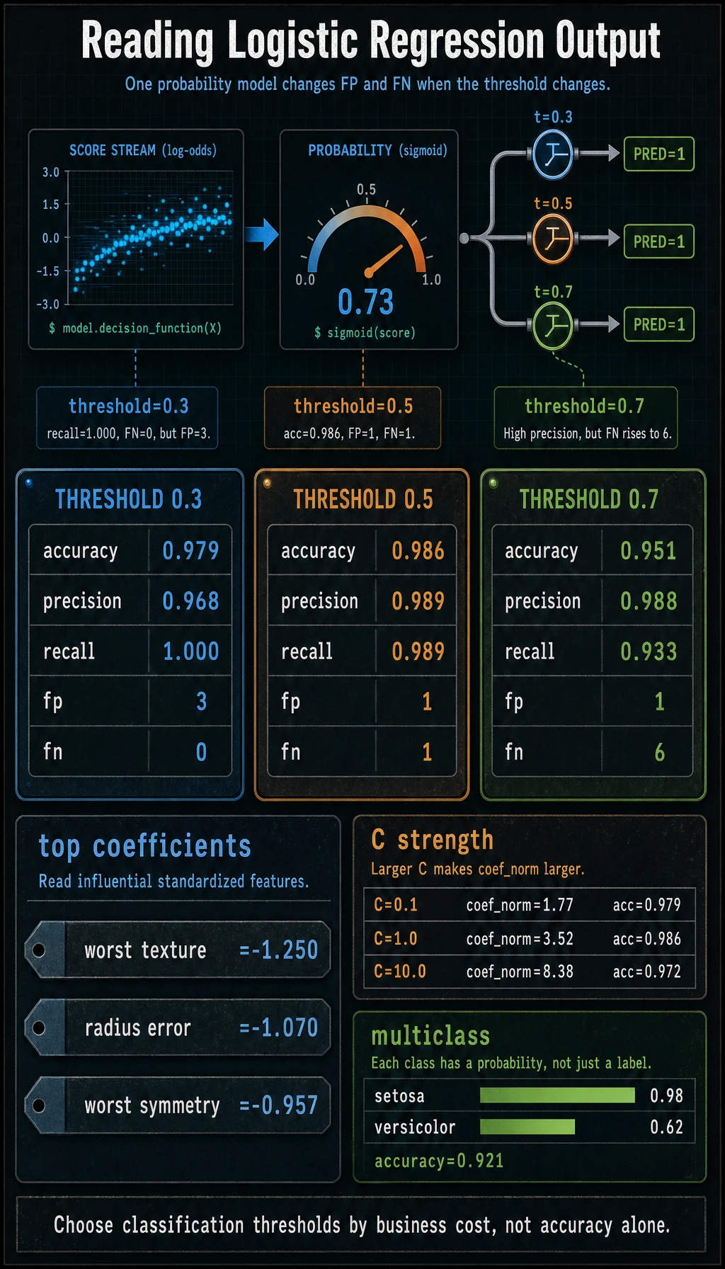

Read the Pipeline

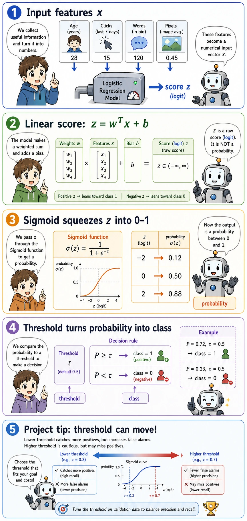
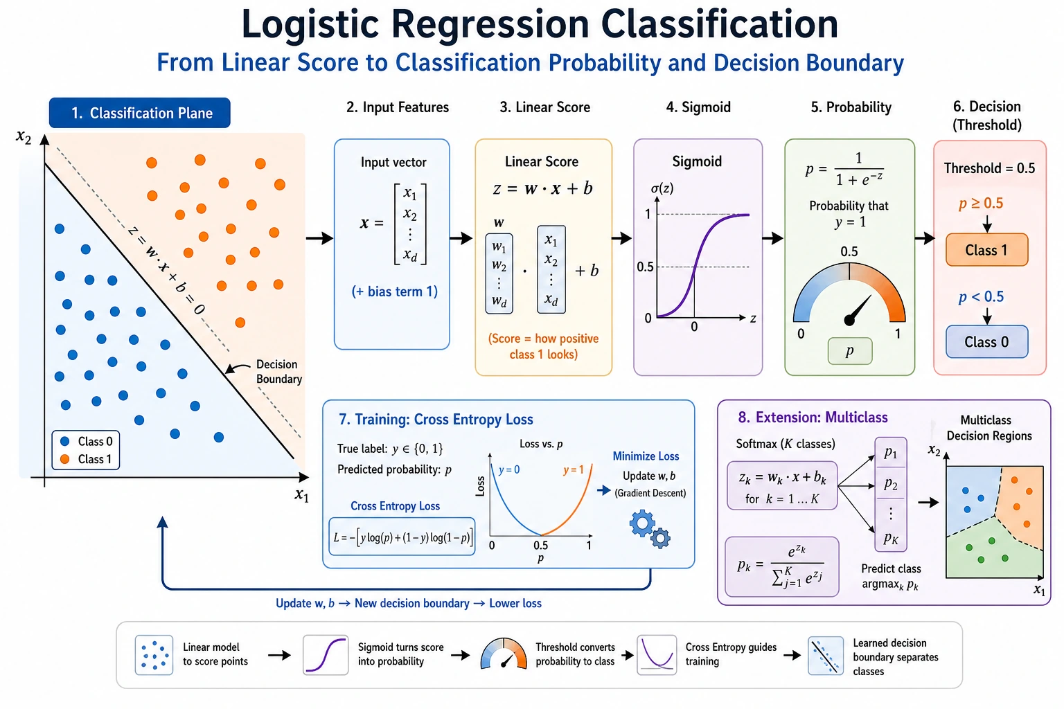
The model is doing three different jobs:

Step	Code	Meaning
Score	z = wT x + b inside LogisticRegression	A raw linear score, not yet a probability
Probability	predict_proba()	The score is converted to a value between 0 and 1
Decision	prob >= threshold	The business rule turns probability into class 0 or 1

The most common beginner mistake is to mix these layers together. In real projects, the model can stay the same while the threshold changes.

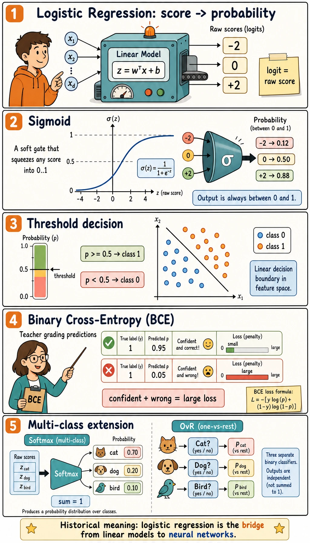
The Minimum Theory You Need

Sigmoid is the function that squeezes any real score into (0, 1):

sigmoid(z) = 1 / (1 + exp(-z))

When z = 0, the probability is 0.5. That is why the default decision boundary for binary logistic regression is the line or hyperplane where the raw score equals zero.

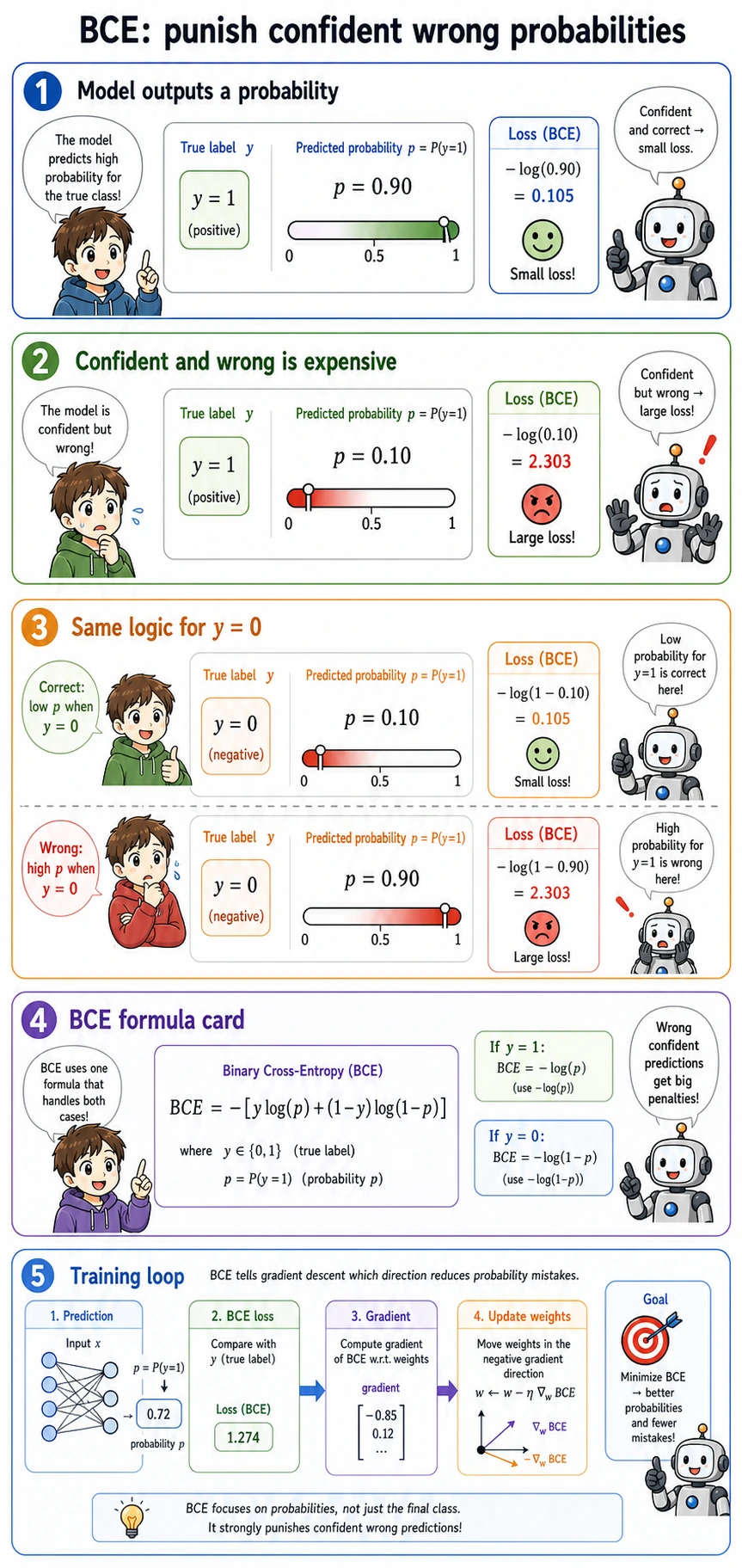
BCE means Binary Cross-Entropy. It is the loss used for binary probability prediction. Its practical rule is simple:

• if the correct answer is 1, predicting 0.99 is excellent and predicting 0.01 is terrible;
• if the correct answer is 0, predicting 0.01 is excellent and predicting 0.99 is terrible;
• confident wrong predictions are punished much more than uncertain wrong predictions.

That is why logistic regression learns probabilities better than forcing linear regression to predict 0 and 1.

Threshold Is a Product Decision

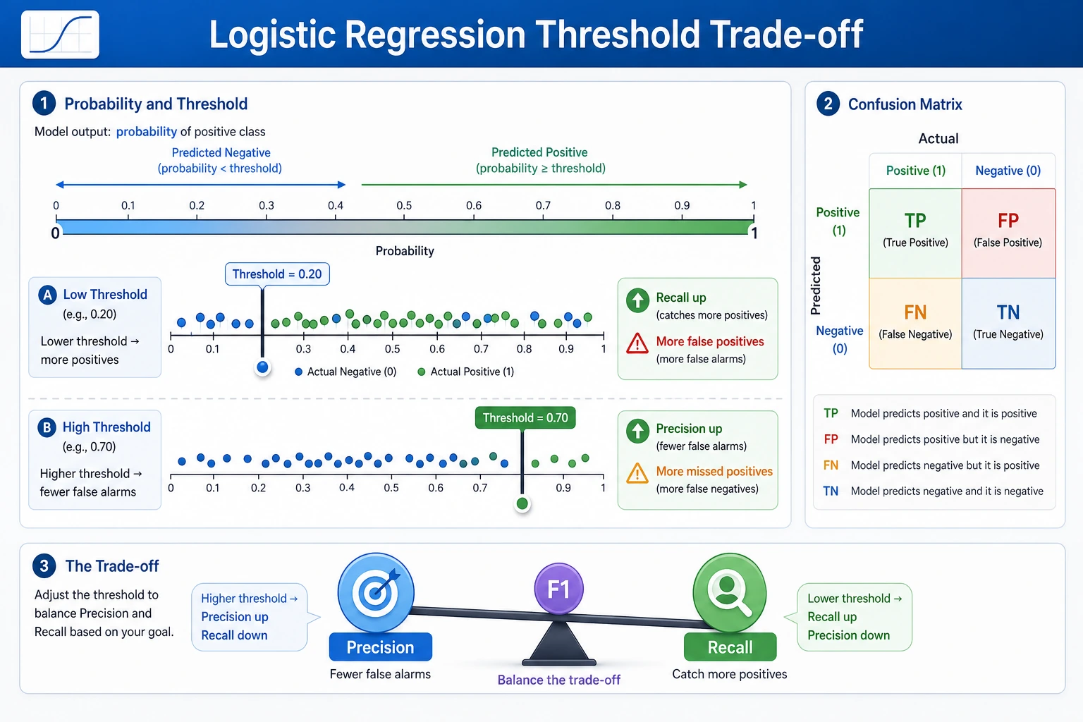
In the output, changing the threshold changes the type of mistake:

Threshold	What happened	When it may be useful
0.3	recall reached 1.000, but false positives increased	Screening, alerting, first-pass filtering
0.5	best balanced score in this split	General default when costs are unknown
0.7	fewer false positives, more false negatives	Expensive manual review, strict confirmation

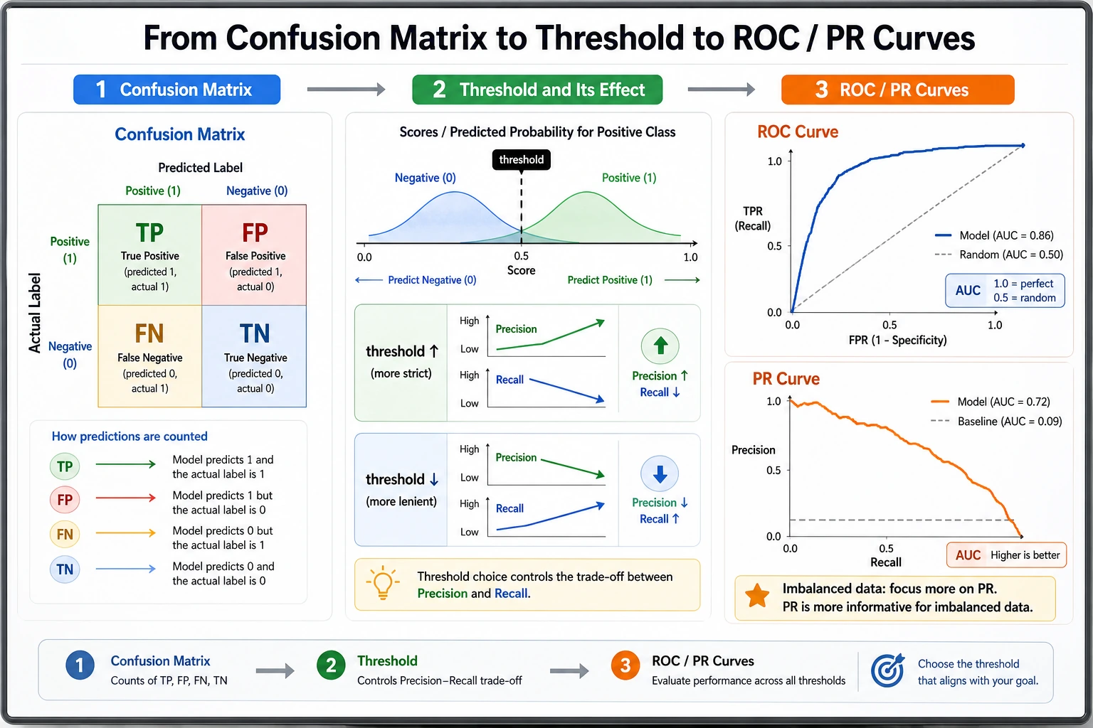
For experienced readers: do not choose the threshold only from accuracy. Check the cost of fp and fn, then compare precision-recall curves or ROC curves.

Regularization and C

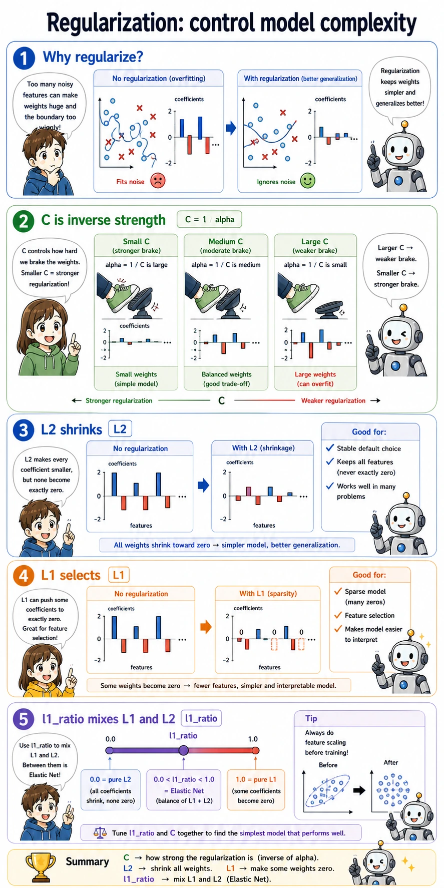
C is the inverse regularization strength in sklearn:

• smaller C means stronger regularization;
• stronger regularization usually creates smaller coefficients;
• very large coefficients can mean the model is trying too hard to fit noise.

The lab output shows this pattern:

C=0.1  accuracy=0.979 coef_norm=1.77
C=1.0  accuracy=0.986 coef_norm=3.52
C=10.0 accuracy=0.972 coef_norm=8.38

The highest coefficient norm is not the best model here. For a production baseline, prefer a model that is accurate, stable, and easy to explain.

Multi-Class Classification

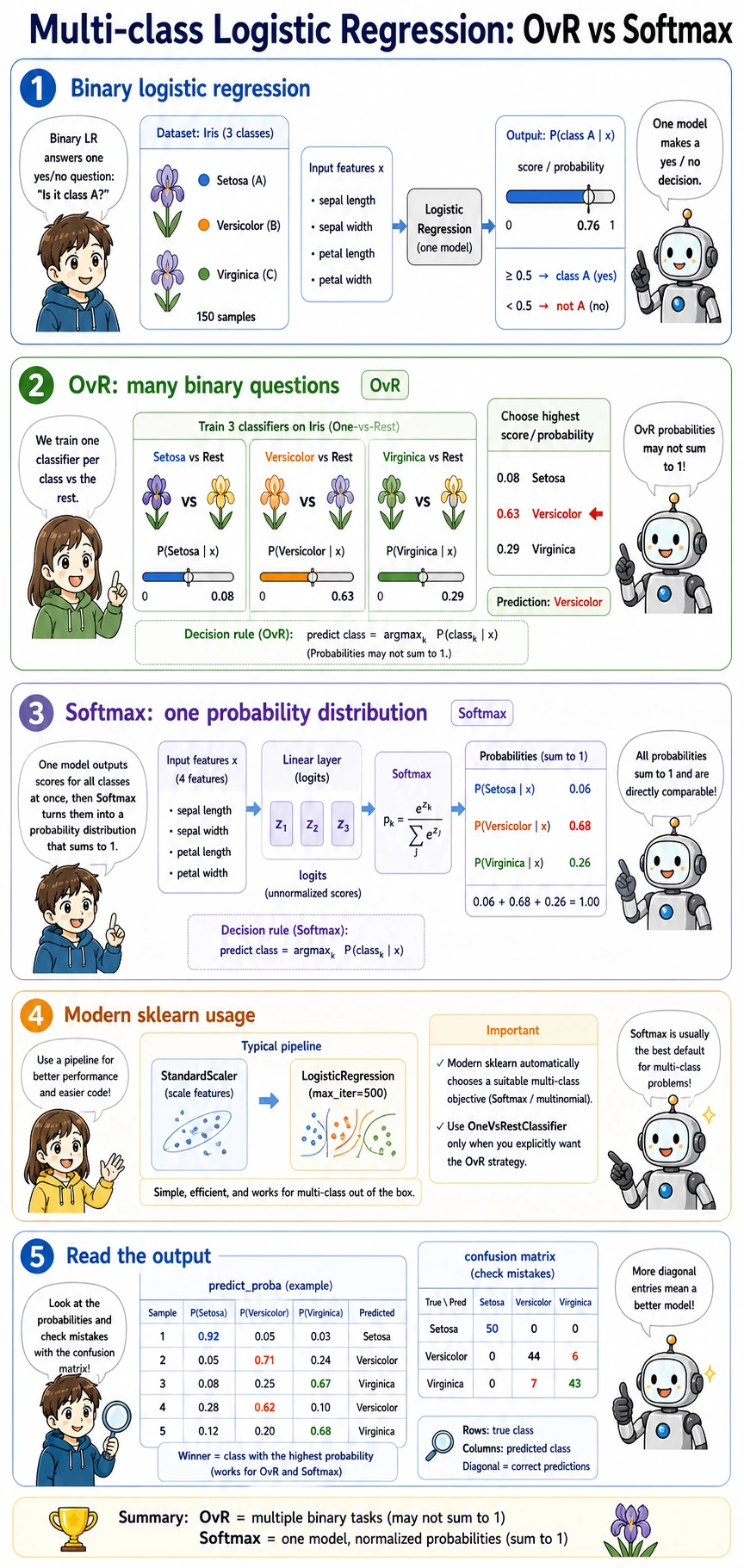
For more than two classes, logistic regression still returns probabilities. In the Iris output, each row sums to about 1.0:

setosa:0.03 | versicolor:0.62 | virginica:0.35

That means the model prefers versicolor, but it is not completely sure. This uncertainty is useful for review queues, active learning, and human-in-the-loop workflows.

Practical Debugging Checklist

Symptom	Likely cause	Fix
Training does not converge	features are not scaled, or max_iter is too small	use StandardScaler in a Pipeline; increase max_iter
Accuracy looks high but recall is poor	class imbalance or wrong threshold	print confusion matrix, precision, recall, F1
Coefficients are hard to compare	features have different units	scale numeric features first
Test score is suspiciously perfect	preprocessing was fitted before the train-test split	keep preprocessing inside Pipeline
Multi-class code warns about old flags	using deprecated multi_class arguments	use the default sklearn behavior unless you need a specific solver

Practice

1. Change the threshold list to [0.2, 0.4, 0.6, 0.8]. Which threshold has the fewest false negatives?
2. Change C to [0.01, 0.1, 1, 10, 100]. When does accuracy stop improving?
3. Print the three smallest coefficients as well as the three largest absolute coefficients. What changes after feature scaling?
4. Replace the breast cancer dataset with your own CSV. Keep the same structure: split first, fit the pipeline, print metrics, tune the threshold.

Reference implementation and walkthrough

1. Lower thresholds usually produce fewer false negatives because more examples are labeled positive. The tradeoff is more false positives, so compare precision and recall together.
2. Accuracy often plateaus after a middle C value. Once validation accuracy stops improving, prefer the simpler or more stable setting.
3. After scaling, coefficients are more comparable because features are on similar units. Coefficients near zero usually have less influence in the fitted linear decision rule.
4. For your own CSV, define the target, split before preprocessing, keep preprocessing inside a Pipeline, then report confusion matrix, precision/recall/F1, and threshold behavior.

Evidence to Keep

Keep this page’s proof of learning as a small evidence card:

Task

regression or classification problem with target definition

Model

linear/logistic/tree/ensemble/SVM configuration and train/test split

Metric

regression error, accuracy/F1, threshold curve, or confusion matrix

Failure Check

overfitting, underfitting, feature scaling, threshold choice, or class imbalance

Expected Output

model result plus error samples or residual review

Pass Check

You have finished this lesson when you can explain these four sentences without looking:

• Logistic regression is a classifier that predicts probabilities.
• predict_proba() gives probabilities; a threshold turns them into labels.
• C controls regularization, and smaller C means stronger regularization.
• Accuracy alone is not enough when false positives and false negatives have different costs.