5.2.2 Linear Regression: Baseline, Residuals, Regularization

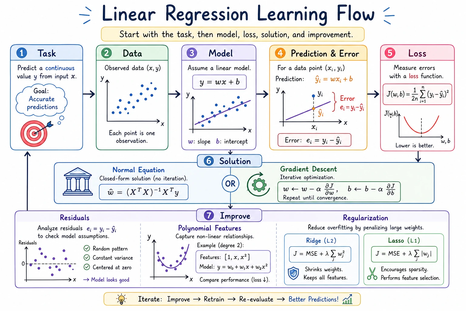
Linear regression answers one practical question: can a few input numbers explain or predict one continuous target number? Examples: price, sales, demand, temperature, latency, or cost.

Look at the Intuition First

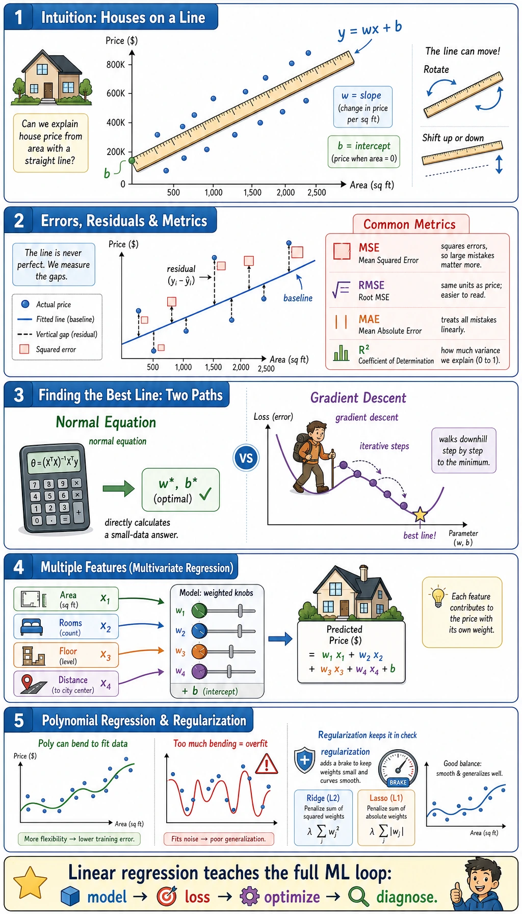
Keep this mental model:

features→weighted sum→prediction→residual→metric→improvement

Word	First meaning
feature	an input column such as area, rooms, age
coefficient	how much the prediction changes when one feature increases
intercept	the base prediction before feature effects are added
residual	true value - predicted value
RMSE	typical error size, penalizing large misses
MAE	typical absolute error, easier to explain
R²	rough percentage of variation explained by the model

Run the Complete Regression Lab

Create ch05_linear_regression_lab.py.

import numpy as np
from sklearn.linear_model import LinearRegression, Ridge
from sklearn.metrics import mean_absolute_error, mean_squared_error, r2_score
from sklearn.model_selection import train_test_split
from sklearn.pipeline import Pipeline
from sklearn.preprocessing import PolynomialFeatures, StandardScaler

rng = np.random.default_rng(42)
area = rng.uniform(45, 180, 80)
rooms = rng.integers(1, 5, 80)
age = rng.uniform(0, 30, 80)
noise = rng.normal(0, 12, 80)
price = 35 + 2.8 * area + 18 * rooms - 1.6 * age + noise
X = np.column_stack([area, rooms, age])

X_train, X_test, y_train, y_test = train_test_split(
    X, price, test_size=0.25, random_state=42
)

baseline = np.full_like(y_test, y_train.mean())
model = LinearRegression()
model.fit(X_train, y_train)
pred = model.predict(X_test)

print("baseline_rmse=", round(mean_squared_error(y_test, baseline) ** 0.5, 2))
print("linear_rmse=", round(mean_squared_error(y_test, pred) ** 0.5, 2))
print("linear_mae=", round(mean_absolute_error(y_test, pred), 2))
print("linear_r2=", round(r2_score(y_test, pred), 3))
print("intercept=", round(model.intercept_, 2))
print("coefficients=", np.round(model.coef_, 2).tolist())
print("first_prediction=", round(pred[0], 2))
print("first_residual=", round(y_test[0] - pred[0], 2))

poly = Pipeline([
    ("poly", PolynomialFeatures(degree=2, include_bias=False)),
    ("scale", StandardScaler()),
    ("ridge", Ridge(alpha=10.0)),
])
poly.fit(X_train, y_train)
poly_pred = poly.predict(X_test)
print("ridge_poly_rmse=", round(mean_squared_error(y_test, poly_pred) ** 0.5, 2))

Run:

python ch05_linear_regression_lab.py

Expected output:

baseline_rmse= 123.23
linear_rmse= 11.68
linear_mae= 8.59
linear_r2= 0.991
intercept= 30.54
coefficients= [2.85, 17.97, -1.72]
first_prediction= 457.07
first_residual= 30.0
ridge_poly_rmse= 13.8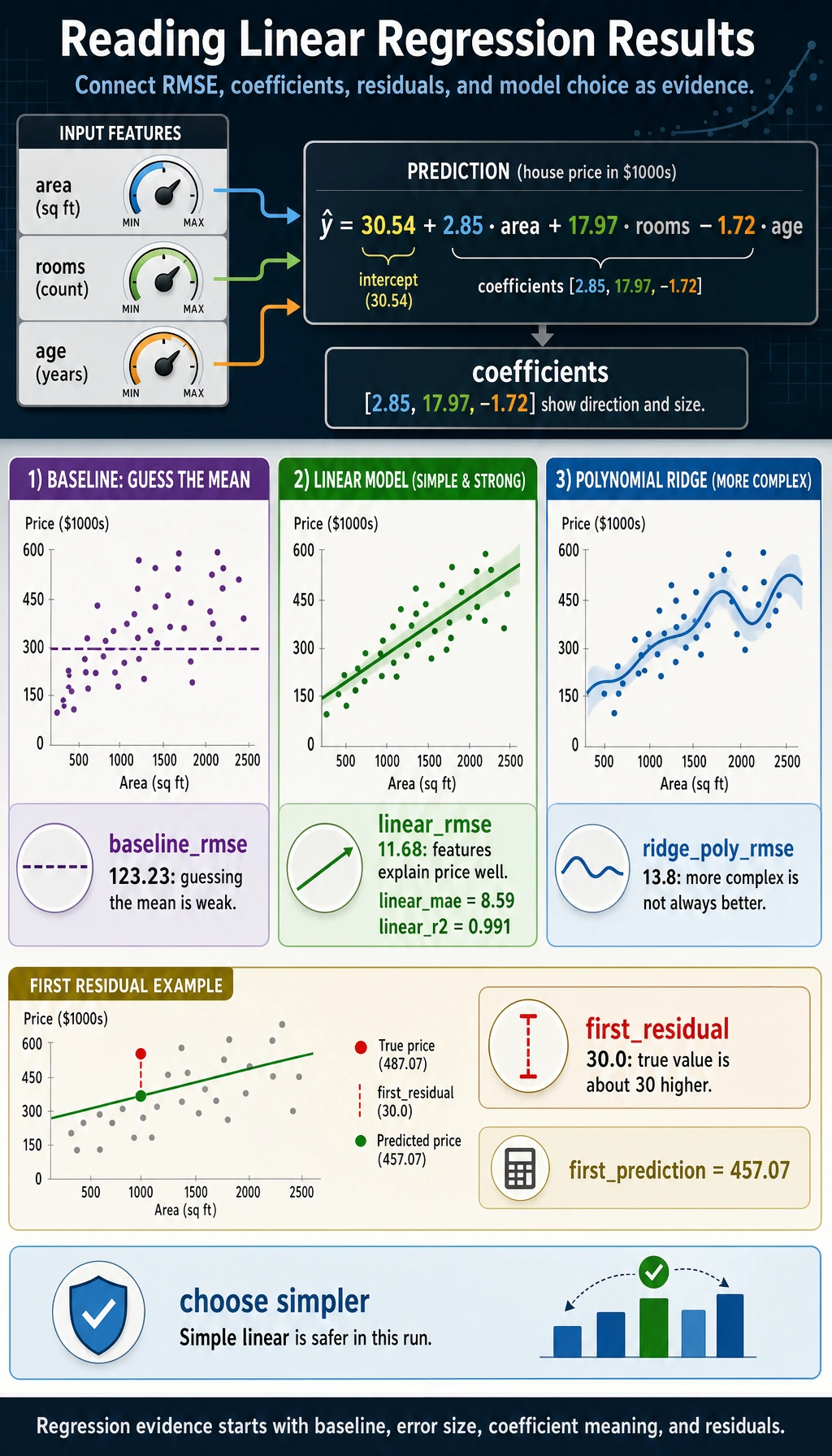

Read the Result

The baseline predicts the training average for every house. Its RMSE is large, so the features matter.

The linear model learns a rule close to the hidden data recipe:

price ~= 30.54 + 2.85 * area + 17.97 * rooms - 1.72 * age

That means, in this synthetic dataset:

Feature	Learned direction	Interpretation
area	positive	larger houses cost more
rooms	positive	more rooms add value
age	negative	older houses cost less

The first residual is 30.0, meaning the first test item was about 30 price units higher than the model predicted. One score is not enough; residuals tell you where the model is weak.

Solver Choice

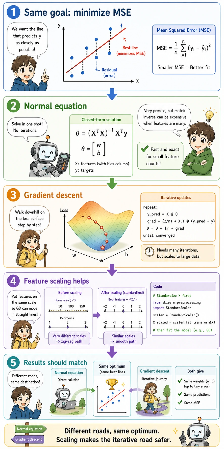
You do not need to hand-solve linear regression every day, but you should know the two ideas:

Solver	What it means	When to care
normal equation / least squares	solve the best coefficients directly	small classic regression, theory intuition
gradient descent	improve coefficients step by step by lowering loss	large data, neural networks, custom objectives

In daily sklearn work, call LinearRegression() first. Learn manual gradient descent to understand later neural networks, not because it is the default production implementation.

Polynomial and Ridge

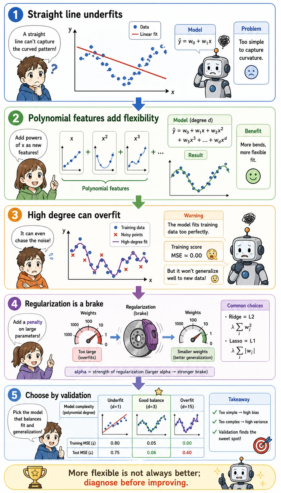
The script also tries:

PolynomialFeatures(degree=2)→StandardScaler→Ridge(alpha=10)

This lets the model use interactions such as area * rooms, but Ridge adds a brake so the model does not bend too freely. In this synthetic run, polynomial Ridge is worse than the simple linear model, so the safer choice is the simpler one.

Check Residuals

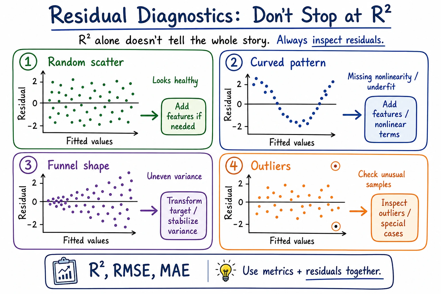
When a regression model looks good, still inspect residuals:

Residual pattern	Meaning	Next action
random around zero	linear model may be enough	keep baseline and document result
curve shape	relationship may be nonlinear	try polynomial/features or another model
bigger spread at high values	error grows with target size	transform target or use robust metrics
a few huge misses	outliers or missing features	review rows and data quality

Evidence to Keep

Keep this page’s proof of learning as a small evidence card:

Task

regression or classification problem with target definition

Model

linear/logistic/tree/ensemble/SVM configuration and train/test split

Metric

regression error, accuracy/F1, threshold curve, or confusion matrix

Failure Check

overfitting, underfitting, feature scaling, threshold choice, or class imbalance

Expected Output

model result plus error samples or residual review

Common Failures

Symptom	First check	Usual fix
model only slightly beats baseline	weak or wrong features	add useful columns, inspect correlations
great R² but bad individual cases	residuals hidden by average score	print largest residuals
coefficient signs feel wrong	feature leakage or correlated features	review columns and domain logic
polynomial model gets worse	overfitting or unstable scale	use Ridge and compare on test data
metrics are confusing	target unit unclear	report MAE/RMSE in business units

Practice

1. Increase noise from 12 to 30 and rerun. What happens to RMSE and R²?
2. Remove age from X. Does the error grow?
3. Change Ridge(alpha=10.0) to alpha=0.1 and alpha=100.0.
4. Save a short note with baseline RMSE, linear RMSE, best model, and one residual example.

Reference implementation and walkthrough

1. More noise should increase RMSE and usually reduce R², because the target contains less predictable signal.
2. If age carries useful information, removing it should increase error. If error barely changes, the feature may be weak or redundant with other columns.
3. Smaller alpha means weaker regularization and coefficients can grow; larger alpha shrinks coefficients and can underfit.
4. A useful note includes the naive baseline, each model’s metric, the chosen model, and one row with actual, predicted, and residual so the metric has a concrete meaning.

Pass Check

You are ready for the next model when you can explain:

• why a baseline is needed before judging a regression model;
• how coefficients, intercept, prediction, and residual connect;
• why RMSE and MAE answer slightly different questions;
• when polynomial features help and when they overfit;
• why a simpler model can beat a more flexible one.