6.5.2 Attention Mechanism

Section Overview

RNNs pass information step by step. Attention lets one token look directly at other tokens and decide which ones matter. This is the core shift behind Transformers.

Learning Objectives

• Explain why attention helps with long-range dependencies.
• Understand Query, Key, and Value through a retrieval analogy.
• Compute scaled dot-product attention by hand.
• Apply a causal mask that prevents future peeking.
• Read nn.MultiheadAttention shapes in PyTorch.

---

Look at Q/K/V First

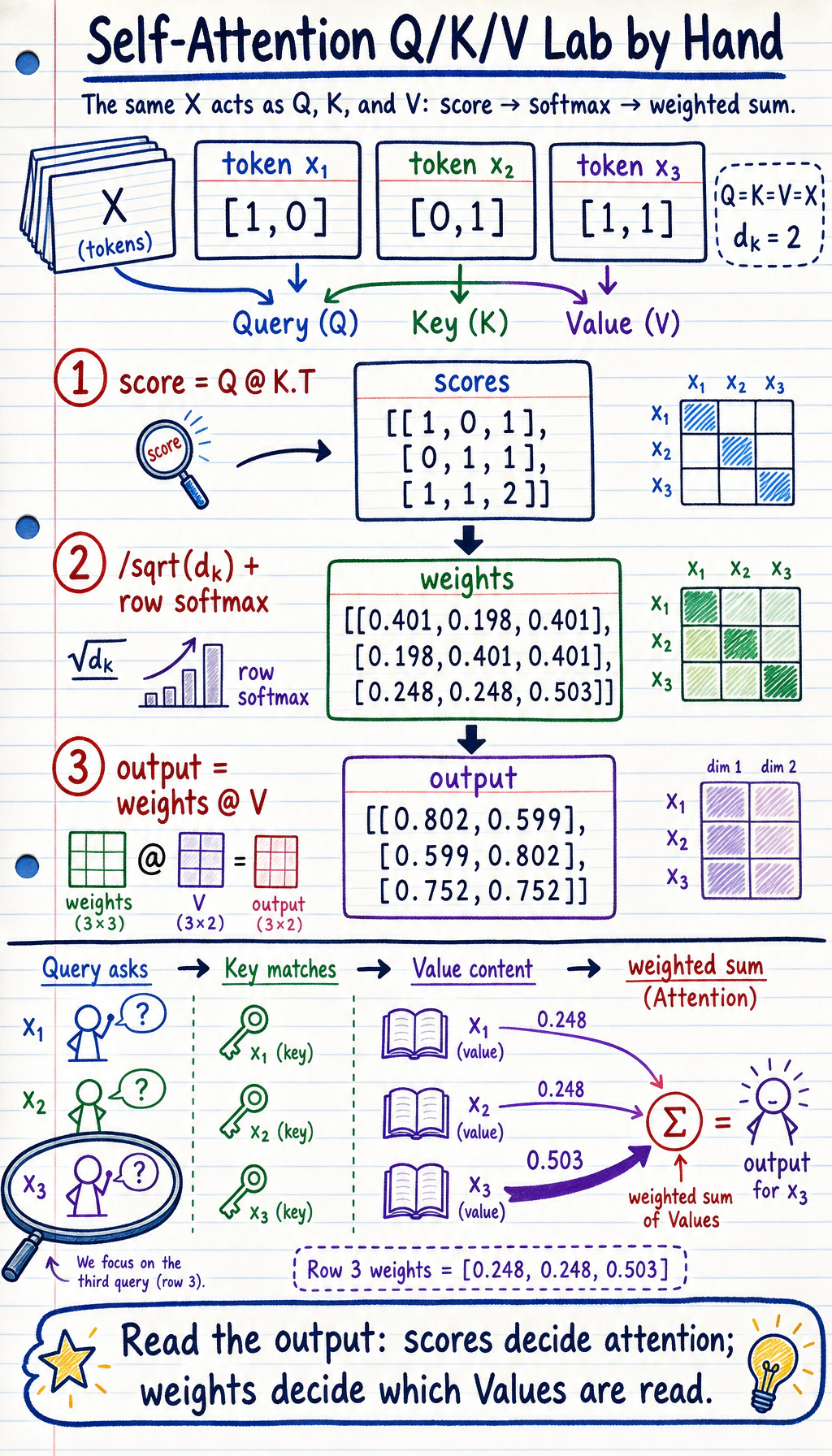
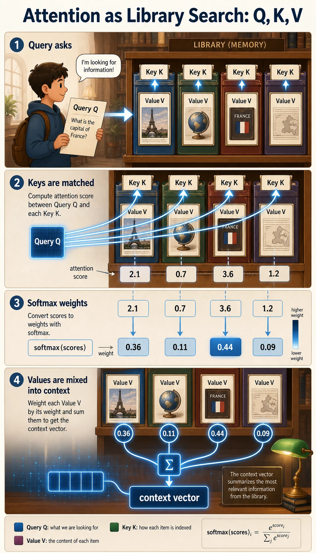
Attention is a weighted retrieval operation:

Q asks→K matches→softmax makes weights→V provides content→weighted sum

The retrieval analogy:

Role	Intuition	In attention
Query Q	what am I looking for?	current token’s question
Key K	what does each item match?	index used for scoring
Value V	what content should be returned?	information that gets mixed

One sentence:

Q scores against K, then the resulting weights mix V.

Why Attention Was Needed

In older sequence models, distant information had to travel through many recurrent steps or be compressed into one fixed vector. Attention shortens the path:

current token→directly scores every token→selects useful context

This gives three practical advantages:

• direct long-range connections;
• better parallel training than step-by-step RNNs;
• a visible matrix of token-to-token mixing weights.

Lab 1: Compute Attention by Hand

For teaching, set Q = K = V = X.

import numpy as np

X = np.array(
    [
        [1.0, 0.0],
        [0.0, 1.0],
        [1.0, 1.0],
    ]
)

Q = K = V = X

scores = Q @ K.T
scaled_scores = scores / np.sqrt(K.shape[1])


def softmax(row):
    e = np.exp(row - row.max())
    return e / e.sum()


weights = np.apply_along_axis(softmax, 1, scaled_scores)
output = weights @ V

print("attention_lab")
print("scores")
print(np.round(scores, 3))
print("weights")
print(np.round(weights, 3))
print("output")
print(np.round(output, 3))

Expected output:

attention_lab
scores
[[1. 0. 1.]
 [0. 1. 1.]
 [1. 1. 2.]]
weights
[[0.401 0.198 0.401]
 [0.198 0.401 0.401]
 [0.248 0.248 0.503]]
output
[[0.802 0.599]
 [0.599 0.802]
 [0.752 0.752]]

Read the three steps:

Step	Code	Meaning
score	Q @ K.T	how strongly each token matches each token
normalize	softmax(...)	convert scores into weights that sum to 1
mix	weights @ V	combine token content according to weights

Lab 1B: Q/K/V Are Learned Views, Not Three Copies

The hand-computation lab used Q = K = V = X so the math stayed visible. A real Transformer usually learns three projection matrices:

Q = XW_q
K = XW_k
V = XW_v

That means the same token representation can be viewed three ways:

• Q: what this position is trying to find;
• K: what this position offers as a match target;
• V: what content this position contributes if selected.

Run this small version:

import numpy as np

X = np.array(
    [
        [1.0, 0.0],
        [0.0, 1.0],
        [1.0, 1.0],
    ]
)

W_q = np.array([[1.0, 0.5], [0.0, 1.0]])
W_k = np.array([[0.5, 1.0], [1.0, 0.0]])
W_v = np.array([[1.0, -0.5], [0.5, 1.0]])

Q = X @ W_q
K = X @ W_k
V = X @ W_v

scores = Q @ K.T / np.sqrt(Q.shape[1])


def softmax(row):
    e = np.exp(row - row.max())
    return e / e.sum()


weights = np.apply_along_axis(softmax, 1, scores)
output = weights @ V

print("projection_lab")
for name, value in [("Q", Q), ("K", K), ("V", V), ("weights", weights), ("output", output)]:
    print(name)
    print(np.round(value, 3))

Expected output:

projection_lab
Q
[[1.  0.5]
 [0.  1. ]
 [1.  1.5]]
K
[[0.5 1. ]
 [1.  0. ]
 [1.5 1. ]]
V
[[ 1.  -0.5]
 [ 0.5  1. ]
 [ 1.5  0.5]]
weights
[[0.248 0.248 0.503]
 [0.401 0.198 0.401]
 [0.284 0.14  0.576]]
output
[[1.128 0.376]
 [1.102 0.198]
 [1.218 0.286]]

Read the evidence:

• Q, K, and V now differ even though they came from the same X.
• The attention weights are computed from Q and K.
• The final output mixes V, not the original X.

This is the main reason Q/K/V should not be memorized as three variable names. They are three learned views that separate matching from content mixing.

Evidence to Keep

Keep one attention trace:

Score Rule

Q @ K.T / sqrt(d_k)

Weights Rule

softmax turns scores into rows that sum to 1

Output Rule

weights @ V mixes value vectors

Qkv Rule

Q/K decide matching, V carries content

Mask Rule

blocked positions receive near-zero attention

Llm Bridge

causal attention lets generation use past tokens only

Why Divide by sqrt(d_k)?

The Transformer formula is:

Attention(Q, K, V) = softmax(QK^T / sqrt(d_k))V

When vectors have many dimensions, dot products can become large. Large scores make softmax too sharp, so one token gets almost all weight. Dividing by sqrt(d_k) cools the scores down and helps training stay stable.

Self-Attention

Self-attention means Q, K, and V all come from the same sequence. Every token can look at every token in that same sequence.

Example question:

"Alex gave Sam the notebook because he trusted him."

To understand “he” and “him,” the current token needs other tokens. Self-attention gives a direct path to them.

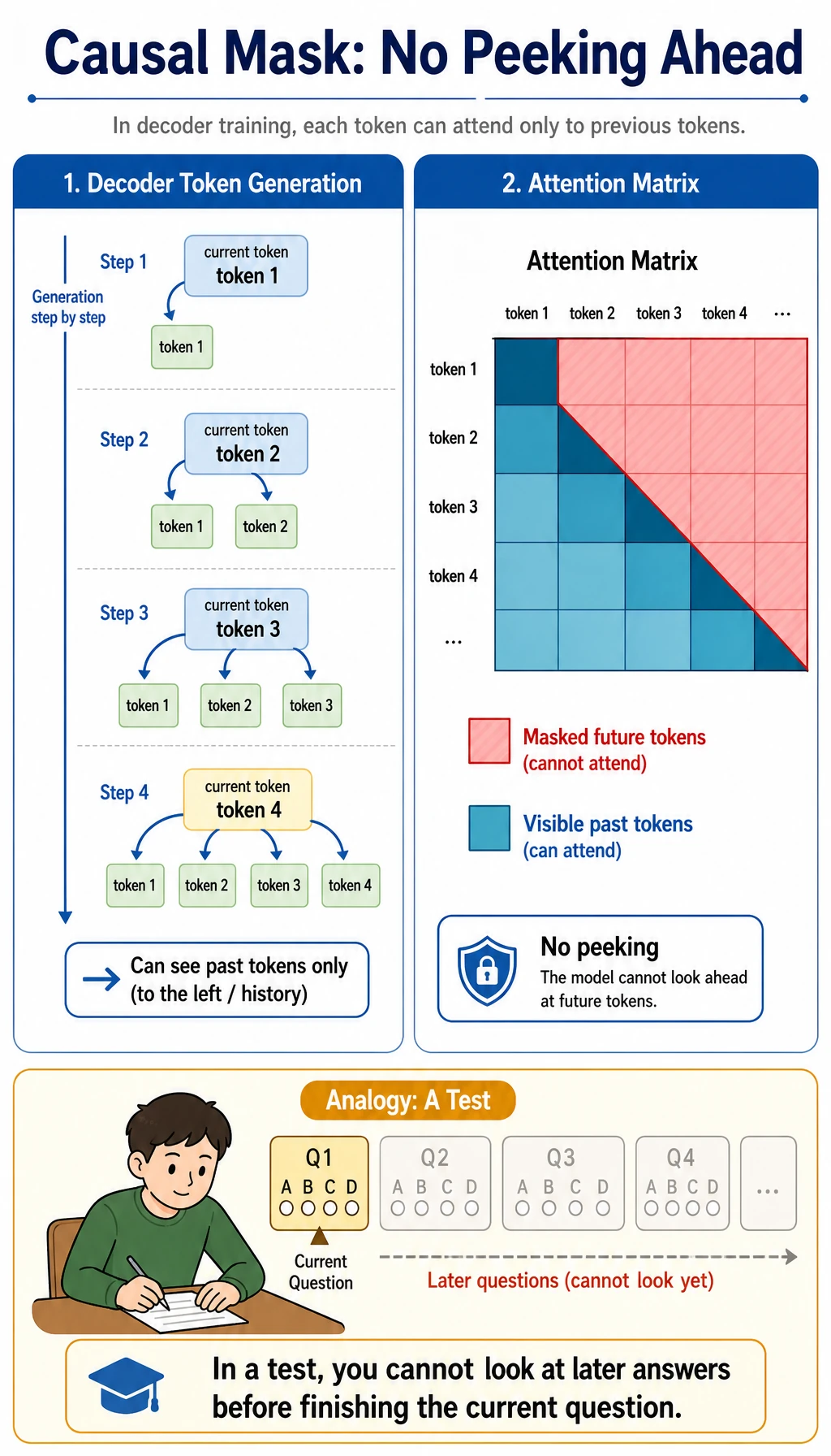
Lab 2: Causal Mask

Generation tasks must not look at future tokens. A causal mask keeps only the lower triangle visible.

import numpy as np

scores = np.array(
    [
        [2.0, 1.0, 0.5],
        [1.2, 2.1, 0.7],
        [0.8, 1.3, 2.2],
    ]
)

mask = np.tril(np.ones_like(scores))
masked_scores = np.where(mask == 1, scores, -1e9)


def softmax(row):
    e = np.exp(row - row.max())
    return e / e.sum()


weights = np.apply_along_axis(softmax, 1, masked_scores)

print("mask_lab")
print(np.round(weights, 3))

Expected output:

mask_lab
[[1.    0.    0.   ]
 [0.289 0.711 0.   ]
 [0.149 0.246 0.605]]

Read it:

• position 1 sees only itself;
• position 2 sees positions 1 and 2;
• position 3 sees positions 1, 2, and 3.

No future answers are visible.

Multi-Head Attention

One attention head can learn one type of relationship. Multi-head attention lets the model inspect several relationship spaces in parallel.

Different heads may focus on:

• nearby position patterns;
• subject/object relationships;
• repeated terms;
• long-range references.

The heads are concatenated and projected back into one representation.

Lab 3: PyTorch MultiheadAttention

import torch
from torch import nn

torch.manual_seed(42)

attention = nn.MultiheadAttention(embed_dim=8, num_heads=2, batch_first=True)
tokens = torch.randn(1, 4, 8)
output, weights = attention(tokens, tokens, tokens)

print("mha_lab")
print("tokens:", tuple(tokens.shape))
print("output:", tuple(output.shape))
print("weights:", tuple(weights.shape))
print("row0_sum:", round(float(weights[0, 0].sum().detach()), 4))

Expected output:

mha_lab
tokens: (1, 4, 8)
output: (1, 4, 8)
weights: (1, 4, 4)
row0_sum: 1.0

Shape reading:

Tensor	Shape	Meaning
tokens	[1, 4, 8]	batch 1, 4 tokens, embedding size 8
output	[1, 4, 8]	each token gets a new context-aware representation
weights	[1, 4, 4]	each query token assigns weights over 4 key tokens

Attention Weights Are Not a Full Explanation

Attention weights are useful, but do not overclaim them.

They tell you:

in this layer/head, this query mixed more value from those key positions

They do not automatically prove:

the model made the final decision because of that token

Use attention weights as a debugging and inspection tool, not as complete causal explanation.

Common Mistakes

Mistake	Fix
treating Q/K/V as mysterious variables	read them as question / index / content
forgetting shape meaning	track [batch, seq_len, embed_dim] and attention [batch, query, key]
using no mask in generation	apply causal mask so future tokens are hidden
applying softmax on the wrong dimension	normalize over key positions
treating attention as reasoning magic	remember score -> softmax -> weighted sum

Exercises

1. Change the third token in Lab 1 to [2.0, 0.0]. How do weights change?
2. In Lab 1B, change only W_v. Which printed values change, and which stay the same?
3. Extend the mask lab to a 4 x 4 matrix.
4. Change num_heads from 2 to 1 in Lab 3. Which shapes stay the same?
5. Explain why attention is easier than a plain RNN for long-distance token interactions.
6. Describe one case where attention weights are useful but not a full explanation.

Reference implementation and walkthrough

1. The changed token becomes more similar to queries that point in the first feature direction, so those queries should give it more attention weight. The exact numbers depend on the full dot-product table.
2. Changing only W_v changes the value vectors and final attention outputs. The attention scores and weights stay the same because they come from queries and keys.
3. A causal 4 x 4 mask should allow each position to see itself and earlier positions while blocking future positions.
4. The final output shape should still be [batch, seq, embed_dim]. What changes is how the model splits the embedding dimension across heads.
5. Attention gives each token a direct path to every other visible token, while a plain RNN must pass information through many sequential steps.
6. Attention weights can suggest which tokens influenced a layer, but they are not a full explanation because value projections, residual paths, later layers, and output heads also shape the final answer.

Key Takeaways

• Attention lets tokens directly select relevant context.
• Q/K/V are learned views that split matching from content retrieval.
• Scaled dot-product attention is score, softmax, weighted sum.
• Causal masks prevent future peeking in generation.
• Multi-head attention views relationships from several subspaces.