7.3.3 Original Transformer vs Modern LLM Decoder

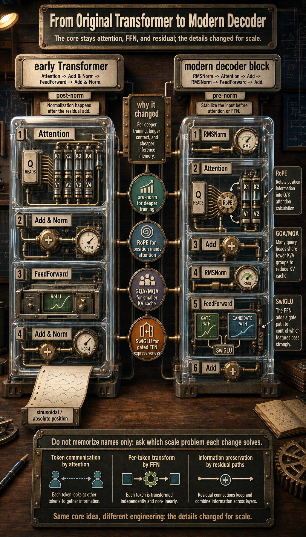
The 2017 Transformer paper gave us the foundation, but most modern LLM decoder blocks are not a line-by-line copy of the original diagram.

The core idea is still the same:

Use attention for token communication, FFN for per-token transformation, and residual paths to preserve information.

But the details have evolved for deeper models, longer contexts, faster inference, and more stable training.

Learning rhythm

Do not memorize the names first. Read the two pipelines as a story: the original block made Transformer work; modern decoder blocks keep the idea but change normalization, position handling, K/V sharing, and FFN design to survive at LLM scale.

The early Transformer block

A simplified early Transformer block is often described as:

Attention→Add & Norm→FeedForward→Add & Norm

Common details include:

• LayerNorm after the residual addition
• sinusoidal or absolute positional encoding
• ordinary Multi-Head Attention
• a ReLU-style feed-forward network in many early descriptions

This structure is still a great learning entry point. It explains the main idea clearly.

But when models become much deeper and serve long conversations, several problems become more visible:

• deep training can become unstable
• absolute positions are less flexible for long context extension
• KV cache becomes expensive during inference
• the FFN needs stronger expressiveness under large-scale training

A common modern LLM decoder block

A simplified modern decoder block often looks more like:

RMSNorm→Attention→Add→RMSNorm→FeedForward→Add

Common details include:

• pre-norm instead of post-norm
• RMSNorm instead of full LayerNorm
• RoPE for position information
• GQA or MQA to reduce KV cache pressure
• SwiGLU-style FFN

This does not mean every modern model is identical. Different models choose different details. But this pattern is common enough that you should recognize it when reading model code.

Pre-norm: normalize before the sublayer

In a post-norm block, the normalization often appears after:

x + sublayer(x)

In a pre-norm block, the sublayer first receives normalized input:

x + sublayer(norm(x))

Why does this matter?

Pre-norm tends to make very deep Transformers easier to train because the residual path stays cleaner. You can think of it as keeping a stable information highway through many layers.

In real code, this is why you often see:

x = x + attention(norm1(x))
x = x + ffn(norm2(x))

RMSNorm: a simpler normalization for scale

LayerNorm normalizes using mean and variance. RMSNorm uses root mean square magnitude and removes the mean-subtraction part.

Beginner-friendly intuition:

• LayerNorm asks: “how far is each value from the average?”
• RMSNorm asks: “how large is this vector overall?”

RMSNorm is popular because it is simpler and efficient while still stabilizing large models well.

You do not need to derive the formula at first. Remember the role:

RMSNorm keeps activations numerically stable with a lighter normalization step.

RoPE: position enters attention by rotation

Early Transformer examples often add positional vectors to token embeddings. Modern LLMs often use:

• RoPE: Rotary Position Embedding

The intuition is:

Instead of adding a position vector once at the input, RoPE rotates Q and K according to position, so relative position information appears inside attention scores.

Why is it useful?

• It works naturally inside attention.
• It gives a good relative-position signal.
• It is often easier to extend or adapt than simple absolute position embeddings.

When you read model code, RoPE usually appears near the attention calculation, before QK^T.

GQA / MQA: reduce KV cache pressure

During inference, decoder-only models cache previous tokens’ K and V. This is called:

• KV cache

Ordinary Multi-Head Attention may store K/V for many heads. Modern serving needs to reduce that memory pressure.

Two common choices are:

Term	Meaning	What it saves
MQA	Multi-Query Attention: many query heads share one K/V group	Maximum K/V sharing
GQA	Grouped-Query Attention: query heads are grouped and share K/V per group	A balance between quality and cache size

Practical intuition:

GQA/MQA do not mainly make the model “smarter.” They make long-context inference cheaper.

SwiGLU FFN: a stronger feed-forward block

The original Transformer FFN is often taught as:

Linear→activation→Linear

Many modern LLMs use a gated FFN such as:

• SwiGLU

The intuition is:

• one path produces candidate features
• another path works like a gate
• the gate decides which features should pass more strongly

You can remember it like this:

SwiGLU lets the FFN not only create features, but also control which features are emphasized.

Run a tiny decoder-block inspection

This script does not implement a full LLM. Its purpose is narrower: connect several architecture words to measurable behavior.

from math import sqrt

activation = [2.0, -1.0, 0.5, 3.0]


def layer_norm(xs, eps=1e-6):
    mean = sum(xs) / len(xs)
    variance = sum((x - mean) ** 2 for x in xs) / len(xs)
    return [(x - mean) / sqrt(variance + eps) for x in xs]


def rms_norm(xs, eps=1e-6):
    rms = sqrt(sum(x * x for x in xs) / len(xs) + eps)
    return [x / rms for x in xs]


decoder_config = {
    "norm": "RMSNorm",
    "position": "RoPE",
    "query_heads": 32,
    "kv_heads": 8,
    "ffn": "SwiGLU",
}

print("LayerNorm:", [round(x, 3) for x in layer_norm(activation)])
print("RMSNorm  :", [round(x, 3) for x in rms_norm(activation)])
print("position :", decoder_config["position"])
print("kv share :", decoder_config["query_heads"] // decoder_config["kv_heads"], "query heads per KV group")
print("ffn style:", decoder_config["ffn"])

Expected output:

LayerNorm: [0.577, -1.402, -0.412, 1.237]
RMSNorm  : [1.06, -0.53, 0.265, 1.589]
position : RoPE
kv share : 4 query heads per KV group
ffn style: SwiGLU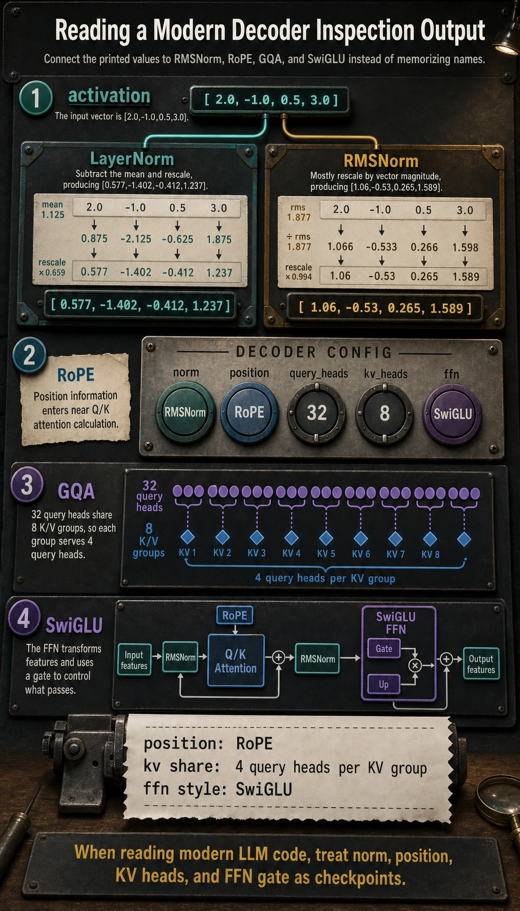

How to read the output

• LayerNorm recenters values around their mean; RMSNorm mostly rescales their magnitude.
• kv share tells you this is GQA: every 4 query heads share one K/V group.
• RoPE and SwiGLU are not decorations. They tell you where position information enters and how the FFN gates features.

A compact comparison table

Part	Early Transformer intuition	Modern LLM decoder intuition
Normalization order	Add & Norm after sublayer	Pre-norm before attention / FFN
Norm type	LayerNorm	Often RMSNorm
Position	Sinusoidal or absolute position	Often RoPE
Attention heads	Ordinary MHA	Often GQA or MQA for inference efficiency
FFN	Basic MLP / ReLU-style	Often SwiGLU gated FFN
Main pressure	Make attention-based sequence modeling work	Scale depth, context, and inference efficiently

How this helps when reading model code

When you open modern model code, do not search only for the word Transformer.

Look for the real components:

• rms_norm
• rotary_emb
• q_proj, k_proj, v_proj
• num_key_value_heads
• gate_proj, up_proj, down_proj

These names are the bridge between the concept diagram and real LLM implementation.

Evidence to Keep

Keep this page’s proof of learning as a small evidence card:

Pre Norm

normalization before attention/FFN for stability

Rmsnorm

scale normalization used in many modern decoders

Rope

position enters attention through rotation

Gqa Mqa

fewer KV heads reduce cache pressure

Swiglu

gated FFN improves capacity at scale

Review notes and pass criteria

• A passing review should map each modern decoder part to the pressure it solves: stability, position, KV cache, or FFN capacity.
• Inspect one real model config and point to num_attention_heads, num_key_value_heads, rotary settings, and FFN projections.
• Keep one confusion note, such as mixing MHA with GQA or treating RoPE as only a positional label. That note becomes the next code-reading target.
• The page is complete when you can read a decoder block diagram and predict which source-code names to search for.

Summary

Modern LLM decoder blocks are not a rejection of the original Transformer.

They are the same idea adapted to harder constraints:

• deeper training
• longer context
• lower latency
• smaller KV cache
• stronger FFN representation

Once you understand these changes, modern LLM architecture diagrams and source code become much less mysterious.