6.2.9 PyTorch + Matplotlib Hands-on Workshop

Learning Rhythm

Use this section as your first complete PyTorch mini-project. The rhythm is: look at the picture → run the code → read the loss curve and decision boundary.

Runtime Environment

If this is your first Station 6 experiment, install the AI dependencies from the project root:

python -m pip install -r requirements-course-ai.txt

For this workshop alone, the minimum extra dependency is torch; matplotlib and scikit-learn are already included in the core course requirements.

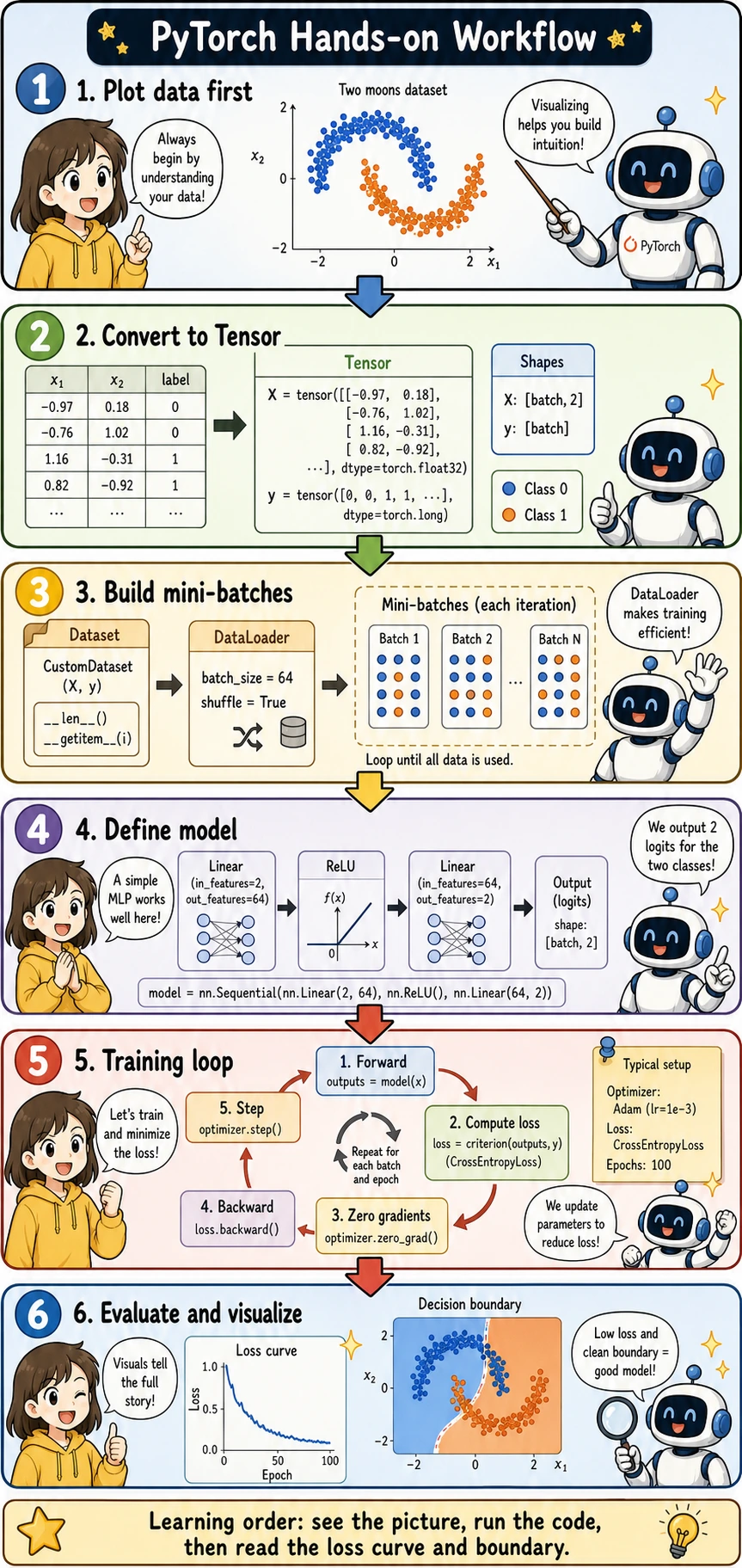
What You Will Build

You will train a small neural network to classify two moon-shaped groups of points. This task is small enough to run quickly, but complete enough to include the core PyTorch workflow:

• Visualize the data with Matplotlib
• Convert NumPy arrays into PyTorch tensors
• Build TensorDataset and DataLoader
• Define an nn.Module
• Train with CrossEntropyLoss and Adam
• Evaluate accuracy
• Plot the loss curve and decision boundary

Keyword Decoder

Term	Beginner-friendly meaning	Why it matters here
Matplotlib	Python’s basic plotting library	Lets you see the dataset, loss curve, and decision boundary
Tensor	PyTorch’s multidimensional array	The model can only train on tensor data
Dataset	Defines what one sample looks like	Keeps data and labels paired correctly
DataLoader	Turns samples into mini-batches	Feeds the training loop batch by batch
MLP	Multilayer Perceptron, a small fully connected neural network	Good first neural network for tabular or 2D toy data
logits	Raw model scores before probability conversion	CrossEntropyLoss expects logits, not softmax probabilities
epoch	One full pass through the training set	Helps you count how many training rounds were completed
decision boundary	The line or region where the model switches class	Makes classification behavior visible

---

Create and Plot the Data First

Before writing a model, always look at the data. This prevents a common beginner mistake: training blindly without knowing what pattern the model is supposed to learn.

import matplotlib.pyplot as plt
from sklearn.datasets import make_moons

X_np, y_np = make_moons(n_samples=600, noise=0.18, random_state=42)

plt.figure(figsize=(6, 5))
plt.scatter(X_np[:, 0], X_np[:, 1], c=y_np, cmap="coolwarm", s=18, alpha=0.8)
plt.xlabel("x1")
plt.ylabel("x2")
plt.title("Two Moons Dataset")
plt.grid(True, alpha=0.3)
plt.show()

What you should notice:

• The two classes are not separable by a straight line
• This is why a small neural network with nonlinearity is useful
• The chart gives you a target picture for the decision boundary later

Convert Data to Tensors

PyTorch models expect tensors. For classification labels used with CrossEntropyLoss, y should be integer class IDs with type torch.long.

import torch

torch.manual_seed(42)

X = torch.tensor(X_np, dtype=torch.float32)
y = torch.tensor(y_np, dtype=torch.long)

print("X shape:", X.shape, "dtype:", X.dtype)
print("y shape:", y.shape, "dtype:", y.dtype)

Expected output:

X shape: torch.Size([600, 2]) dtype: torch.float32
y shape: torch.Size([600]) dtype: torch.int64

The meaning of the shapes is:

• X: [batch, features], and each sample has 2 features
• y: [batch], and each value is a class label: 0 or 1

Build Dataset and DataLoader

TensorDataset keeps X and y paired. DataLoader shuffles the data and creates mini-batches.

from torch.utils.data import DataLoader, TensorDataset, random_split

dataset = TensorDataset(X, y)
train_dataset, val_dataset = random_split(
    dataset,
    [480, 120],
    generator=torch.Generator().manual_seed(42)
)

train_loader = DataLoader(
    train_dataset,
    batch_size=64,
    shuffle=True,
    generator=torch.Generator().manual_seed(7)
)
val_loader = DataLoader(val_dataset, batch_size=128, shuffle=False)

batch_x, batch_y = next(iter(train_loader))
print("batch_x shape:", batch_x.shape)
print("batch_y shape:", batch_y.shape)

Expected output:

batch_x shape: torch.Size([64, 2])
batch_y shape: torch.Size([64])

Why this matters:

• batch_size=64 means the model updates after seeing 64 samples
• shuffle=True prevents the model from always seeing samples in the same order
• Validation data does not need shuffling because it is only used for evaluation

Define a Small Neural Network

This model maps a 2D point to two logits, one score for each class.

from torch import nn

class MoonClassifier(nn.Module):
    def __init__(self):
        super().__init__()
        self.net = nn.Sequential(
            nn.Linear(2, 32),
            nn.ReLU(),
            nn.Linear(32, 32),
            nn.ReLU(),
            nn.Linear(32, 2),
        )

    def forward(self, x):
        return self.net(x)

model = MoonClassifier()
print(model)

Expected output:

MoonClassifier(
  (net): Sequential(
    (0): Linear(in_features=2, out_features=32, bias=True)
    (1): ReLU()
    (2): Linear(in_features=32, out_features=32, bias=True)
    (3): ReLU()
    (4): Linear(in_features=32, out_features=2, bias=True)
  )
)

Important detail:

• The final layer outputs 2 values because this is a two-class task
• Do not add Softmax here because nn.CrossEntropyLoss() expects raw logits

Train and Validate

The training loop follows the same rhythm you saw earlier:

forward → loss → zero_grad → backward → step

loss_fn = nn.CrossEntropyLoss()
optimizer = torch.optim.Adam(model.parameters(), lr=0.01)

train_losses = []
val_losses = []
val_accuracies = []

for epoch in range(1, 101):
    model.train()
    train_loss_sum = 0.0

    for batch_x, batch_y in train_loader:
        logits = model(batch_x)
        loss = loss_fn(logits, batch_y)

        optimizer.zero_grad()
        loss.backward()
        optimizer.step()

        train_loss_sum += loss.item() * len(batch_x)

    train_loss = train_loss_sum / len(train_dataset)
    train_losses.append(train_loss)

    model.eval()
    val_loss_sum = 0.0
    correct = 0

    with torch.no_grad():
        for batch_x, batch_y in val_loader:
            logits = model(batch_x)
            loss = loss_fn(logits, batch_y)
            val_loss_sum += loss.item() * len(batch_x)

            pred = logits.argmax(dim=1)
            correct += (pred == batch_y).sum().item()

    val_loss = val_loss_sum / len(val_dataset)
    val_acc = correct / len(val_dataset)
    val_losses.append(val_loss)
    val_accuracies.append(val_acc)

    if epoch == 1 or epoch % 20 == 0:
        print(
            f"epoch={epoch:3d}, "
            f"train_loss={train_loss:.4f}, "
            f"val_loss={val_loss:.4f}, "
            f"val_acc={val_acc:.1%}"
        )

Expected output:

epoch=  1, train_loss=0.5568, val_loss=0.3786, val_acc=84.2%
epoch= 20, train_loss=0.0755, val_loss=0.1064, val_acc=98.3%
epoch= 40, train_loss=0.0719, val_loss=0.1260, val_acc=98.3%
epoch= 60, train_loss=0.0657, val_loss=0.1290, val_acc=98.3%
epoch= 80, train_loss=0.0655, val_loss=0.1415, val_acc=98.3%
epoch=100, train_loss=0.0687, val_loss=0.1370, val_acc=98.3%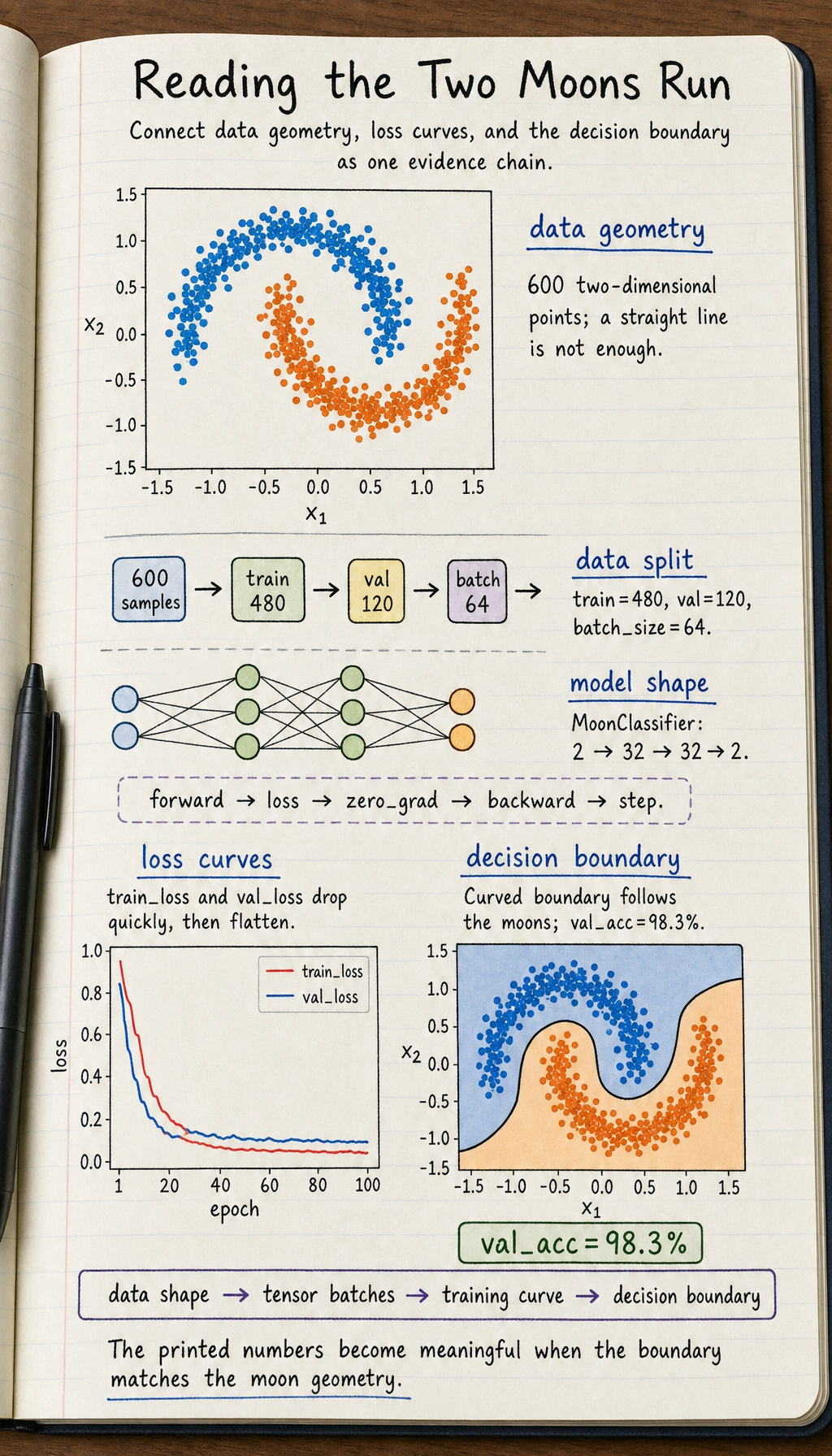

If your exact numbers are slightly different, that is fine. The important sign is that validation accuracy rises clearly above random guessing.

Plot the Loss Curve

The loss curve tells you whether training is moving in the right direction.

plt.figure(figsize=(7, 4))
plt.plot(train_losses, label="train loss")
plt.plot(val_losses, label="validation loss")
plt.xlabel("Epoch")
plt.ylabel("Loss")
plt.title("Training and Validation Loss")
plt.legend()
plt.grid(True, alpha=0.3)
plt.show()

How to read it:

• If both losses decrease, training is learning normally
• If training loss decreases but validation loss rises, watch for overfitting
• If neither decreases, check learning rate, labels, model output shape, and loss function

Plot the Decision Boundary

The decision boundary shows what the model has learned geometrically.

import numpy as np

x_min, x_max = X_np[:, 0].min() - 0.5, X_np[:, 0].max() + 0.5
y_min, y_max = X_np[:, 1].min() - 0.5, X_np[:, 1].max() + 0.5
xx, yy = np.meshgrid(
    np.linspace(x_min, x_max, 250),
    np.linspace(y_min, y_max, 250)
)

grid = np.c_[xx.ravel(), yy.ravel()]
grid_tensor = torch.tensor(grid, dtype=torch.float32)

model.eval()
with torch.no_grad():
    logits = model(grid_tensor)
    grid_pred = logits.argmax(dim=1).numpy().reshape(xx.shape)

plt.figure(figsize=(7, 5))
plt.contourf(xx, yy, grid_pred, alpha=0.25, cmap="coolwarm")
plt.scatter(X_np[:, 0], X_np[:, 1], c=y_np, cmap="coolwarm", s=16, edgecolors="k", linewidths=0.2)
plt.xlabel("x1")
plt.ylabel("x2")
plt.title(f"Decision Boundary (validation accuracy {val_accuracies[-1]:.1%})")
plt.grid(True, alpha=0.2)
plt.show()

This picture is usually the moment when PyTorch starts to feel concrete: the model is no longer just printing numbers; you can see how it divides the space.

Evidence to Keep

Save these four artifacts from the workshop:

Data Plot

shows the original class pattern

Loss Curve

shows whether training and validation improve together

Decision Boundary

shows what the model learned geometrically

Failure Note

one case where the boundary or validation curve looks wrong

If you can explain all four, this workshop has become a training evidence pack rather than a copied notebook.

Common Errors and Fixes

Symptom	Likely cause	Fix
expected scalar type Long	Labels are not torch.long	Use y = torch.tensor(y_np, dtype=torch.long)
Loss does not decrease	Learning rate too large or too small	Try lr=0.001 or lr=0.01
Shape error in loss	Output or label shape is wrong	For CrossEntropyLoss, logits should be [batch, classes], labels should be [batch]
Validation uses too much memory	Gradients are recorded during validation	Use model.eval() and with torch.no_grad()

Practice Tasks

1. Change the hidden size from 32 to 16 and 64. Compare the decision boundary.
2. Change noise=0.18 to noise=0.3. Observe how the task becomes harder.
3. Change the optimizer from Adam to SGD. Compare the loss curve.
4. Add a third hidden layer and check whether validation loss improves or overfits.

Operation guide and checkpoints

1. Hidden size 16 may produce a simpler boundary; 64 can fit a more flexible boundary but may overfit. Use validation loss and the boundary plot together.
2. Higher noise should make the classes overlap more. Expect lower validation accuracy, a less clean boundary, or more uncertain samples near the class border.
3. SGD often needs a more careful learning rate and may converge more slowly than Adam. A slower curve is not a bug if validation keeps improving.
4. A third hidden layer is useful only if validation improves. If train loss improves but validation gets worse, the extra layer is memorizing noise.

Passing Standard

After finishing this workshop, you should be able to explain a complete PyTorch workflow in your own words:

Data picture → Tensor → DataLoader → model → loss → optimizer → training loop → validation → visualization.

If you can also read the loss curve and decision boundary, you are no longer just copying PyTorch code. You are starting to understand what the training process is doing.