6.1.4 Forward and Backward Propagation

Section Overview

Training a neural network is a loop: predict, measure error, compute gradients, update parameters, repeat.

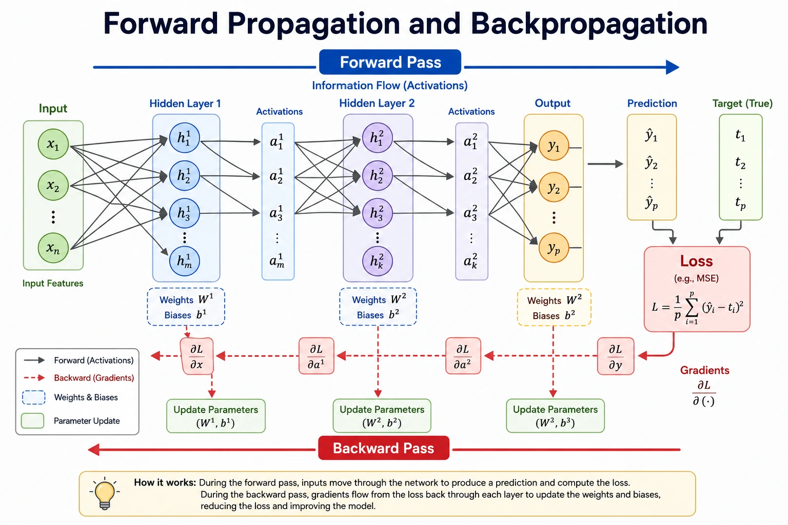
What You Will Build

This lesson runs one tiny PyTorch example that shows:

• a forward pass;
• binary cross-entropy loss;
• gradients created by loss.backward();
• parameter updates created by optimizer.step();
• a mini training loop with decreasing loss.

Setup

python -m pip install -U torch

Run the Complete Lab

Create forward_backward_lab.py:

import torch
import torch.nn as nn


torch.manual_seed(42)

x = torch.tensor([[1.0, 2.0]])
y = torch.tensor([[1.0]])
model = nn.Sequential(nn.Linear(2, 1), nn.Sigmoid())
loss_fn = nn.BCELoss()
optimizer = torch.optim.SGD(model.parameters(), lr=0.5)

print("one_training_step")
with torch.no_grad():
    before = model(x)
print("prediction_before=", round(float(before.item()), 3))

pred = model(x)
loss = loss_fn(pred, y)
optimizer.zero_grad()
loss.backward()

linear = model[0]
print("loss_before=", round(float(loss.item()), 4))
print("weight_grad=", [[round(float(v), 4) for v in row] for row in linear.weight.grad.tolist()])
print("bias_grad=", [round(float(v), 4) for v in linear.bias.grad.tolist()])
optimizer.step()

with torch.no_grad():
    after = model(x)
    new_loss = loss_fn(after, y)
print("prediction_after=", round(float(after.item()), 3))
print("loss_after=", round(float(new_loss.item()), 4))

print("mini_training_loop")
for step in range(1, 6):
    pred = model(x)
    loss = loss_fn(pred, y)
    optimizer.zero_grad()
    loss.backward()
    optimizer.step()
    print(f"step={step} loss={loss.item():.4f} pred={pred.item():.3f}")

Run it:

python forward_backward_lab.py

Expected output:

one_training_step
prediction_before= 0.825
loss_before= 0.1927
weight_grad= [[-0.1753, -0.3505]]
bias_grad= [-0.1753]
prediction_after= 0.888
loss_after= 0.1183
mini_training_loop
step=1 loss=0.1183 pred=0.888
step=2 loss=0.0861 pred=0.918
step=3 loss=0.0678 pred=0.934
step=4 loss=0.0560 pred=0.945
step=5 loss=0.0478 pred=0.953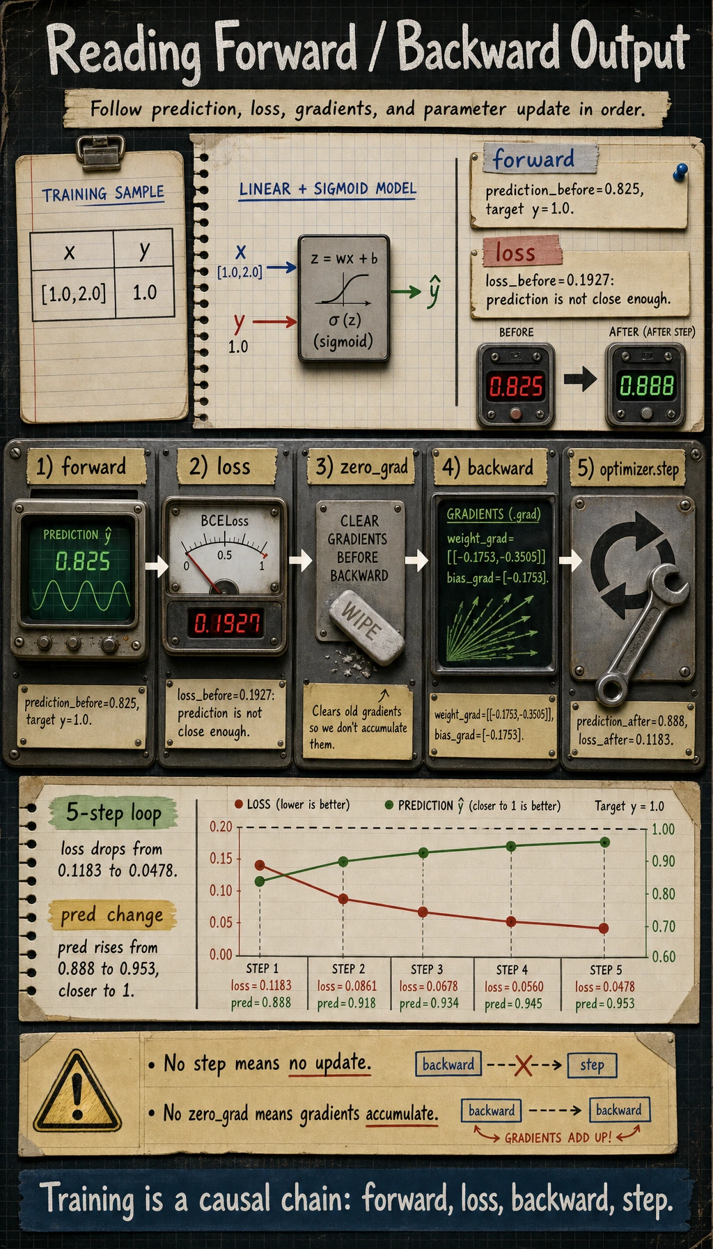

Read the Five Steps

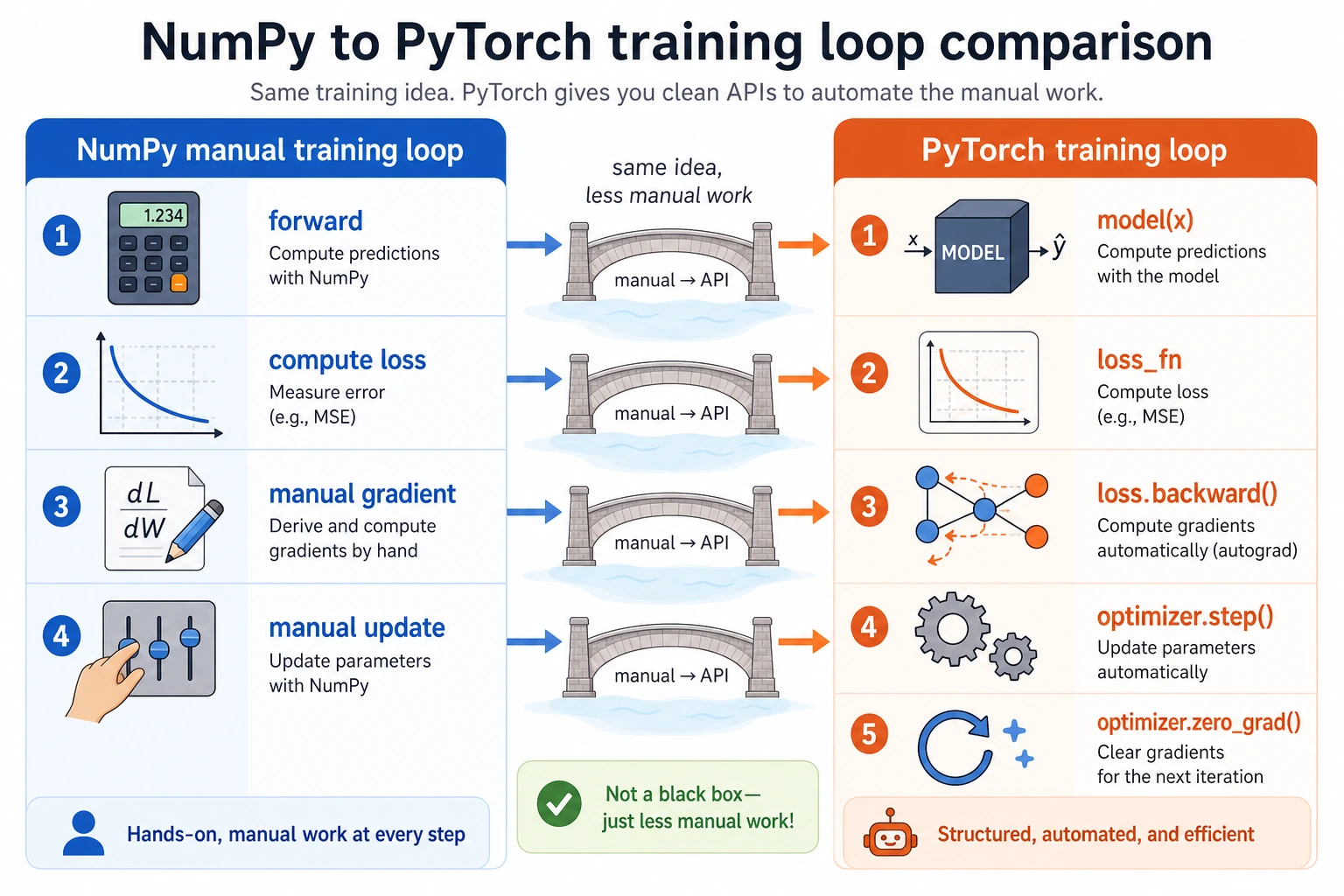
One training step has a fixed order:

Step	Code	Meaning
forward	pred = model(x)	compute prediction
loss	loss = loss_fn(pred, y)	measure error
clear	optimizer.zero_grad()	remove old gradients
backward	loss.backward()	compute gradients
update	optimizer.step()	change parameters

The order matters. If you forget zero_grad(), gradients accumulate from previous steps. If you forget step(), the model never updates.

Forward Propagation

Forward propagation means data moves from input to output:

pred = model(x)

Here the model is:

nn.Sequential(nn.Linear(2, 1), nn.Sigmoid())

The linear layer computes a score, and Sigmoid turns it into a probability-like value.

Loss Function

The target is 1.0, and the prediction starts at 0.825, so the model is close but not perfect:

loss_before= 0.1927

BCELoss means binary cross-entropy. It is suitable here because the output is a binary probability after Sigmoid.

For later PyTorch work, remember this pairing:

Output style	Loss
final Sigmoid probability	nn.BCELoss()
raw logits without Sigmoid	nn.BCEWithLogitsLoss()
multi-class raw logits	nn.CrossEntropyLoss()

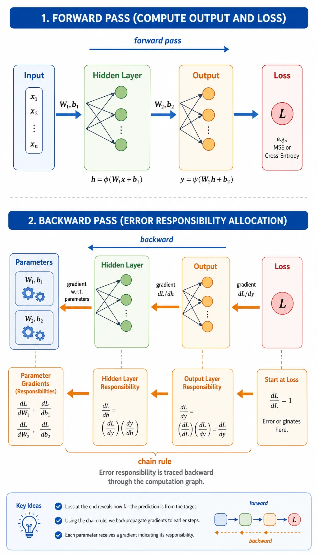
Backward Propagation

loss.backward() fills gradient fields:

weight_grad= [[-0.1753, -0.3505]]
bias_grad= [-0.1753]

A gradient tells the optimizer how changing a parameter would change the loss. You do not manually derive every gradient in PyTorch; autograd builds the computation graph during forward pass and uses it during backward pass.

Optimizer Step

After optimizer.step(), the prediction moves closer to the target:

prediction_before= 0.825
prediction_after= 0.888
loss_after= 0.1183

That is training in miniature: parameters changed, the prediction improved, and loss decreased.

Evidence to Keep

Save one before/after record:

Prediction Before

0.825

Loss Before

0.1927

Gradient Seen

weight_grad and bias_grad are not None

Prediction After

0.888

Loss After

0.1183

This proves the full training step happened. If any one line is missing, debug in this order: forward output, loss, gradient, optimizer update.

Practical Debugging Checklist

Symptom	Likely cause	Fix
loss never changes	forgot optimizer.step()	call step() after backward()
gradients keep growing strangely	forgot zero_grad()	clear gradients every step
grad is None	tensor not connected to loss or no backward()	check computation graph
binary loss errors	output/target shape mismatch	make both [batch, 1] here
loss becomes nan	learning rate too high or invalid values	lower LR, inspect inputs

Practice

1. Change lr=0.5 to 0.05 and 1.0. How does loss change?
2. Remove optimizer.zero_grad() and print gradients. What accumulates?
3. Replace nn.BCELoss() with nn.BCEWithLogitsLoss() and remove nn.Sigmoid().
4. Add another sample to x and y, then verify shapes.
5. Print model weights before and after optimizer.step().

Reference implementation and walkthrough

1. lr=0.05 usually updates more slowly, while lr=1.0 may improve quickly or overshoot. The loss curve is the evidence, not the learning rate number alone.
2. If optimizer.zero_grad() is removed, gradients accumulate across backward calls. The printed gradients become a sum of old and new signals instead of the current batch signal.
3. BCEWithLogitsLoss expects raw logits and applies the numerically stable sigmoid-plus-BCE calculation internally. Keeping an explicit Sigmoid would apply that squashing twice.
4. After adding a sample, the first dimension of x, y, predictions, and loss input must still match. Shape mismatches usually mean the data and target were not expanded together.
5. After optimizer.step(), at least one weight or bias should change. If nothing changes, check requires_grad, loss.backward(), the optimizer parameter list, and the learning rate.

Pass Check

You are done when you can explain:

• forward pass computes predictions;
• loss measures error;
• backward pass computes gradients;
• optimizer step updates parameters;
• zero_grad() prevents old gradients from accumulating.