4.2.4 Basics of Statistical Inference

Statistical inference = inferring rules from data

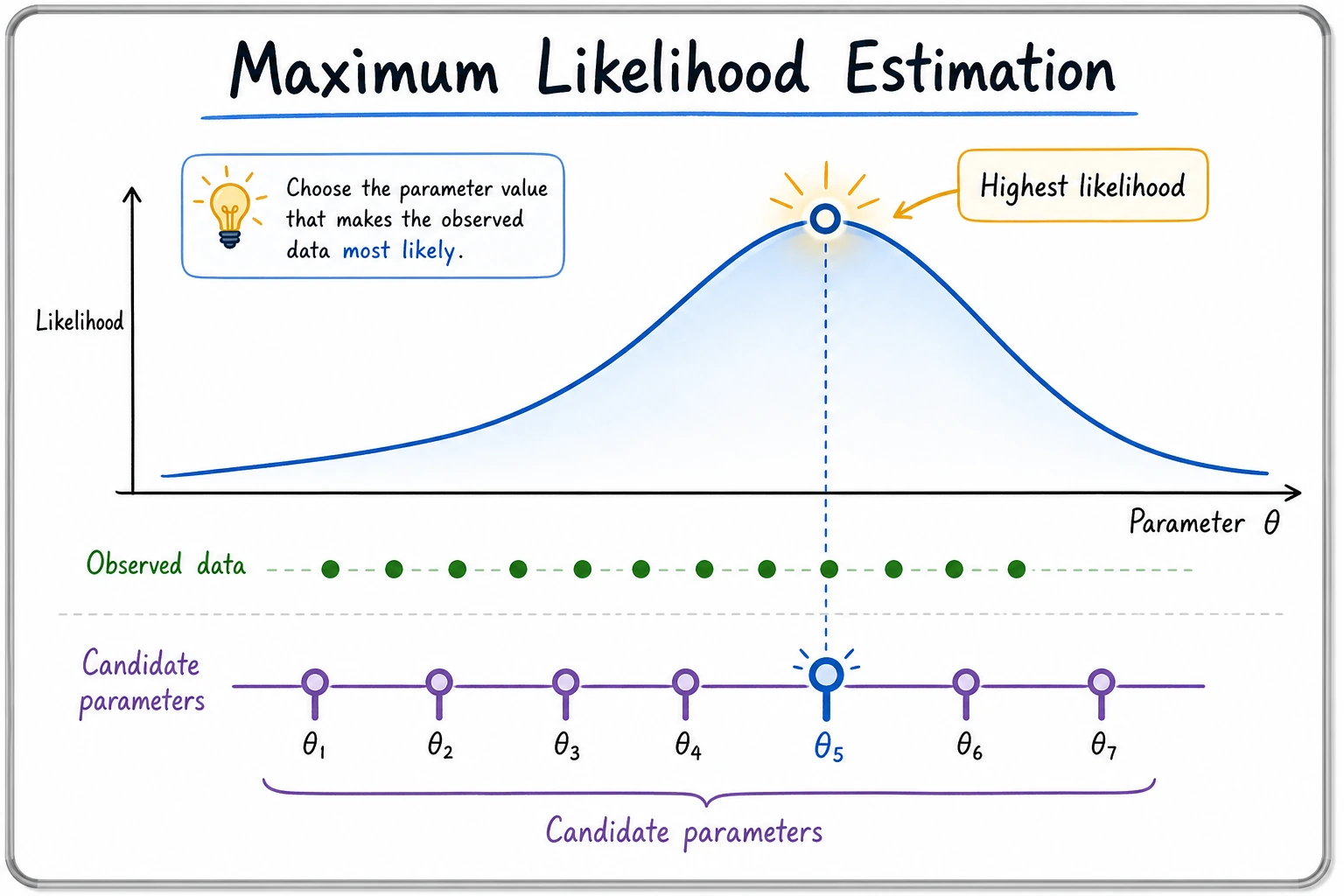
In the previous section, we learned about various probability distributions. But in the real world, we often do not know the parameters of a distribution (for example, what is the probability that a coin lands heads?). Statistical inference is using observed data to infer the parameters of the distribution.

Learning Objectives

• Understand the intuition behind Maximum Likelihood Estimation (MLE) — why do we “maximize probability”?
• Understand Maximum A Posteriori Estimation (MAP) — adding prior knowledge
• Understand hypothesis testing and p-values (A/B testing mindset)
• Implement MLE in Python

Terms to Decode Before Inference

Statistical inference has many compact terms. Read them as a workflow rather than as isolated definitions:

Term	Full name / meaning	Beginner-friendly question
MLE	Maximum Likelihood Estimation	Which parameters make the observed data most likely?
MAP	Maximum A Posteriori	Which parameters are most plausible after combining data and prior belief?
EM	Expectation-Maximization	If some variables are hidden, how can we alternately guess them and update parameters?
likelihood	Probability of data under a parameter	If this parameter were true, how likely would this dataset be?
log-likelihood	Log of likelihood	A numerically stable way to add many probability terms instead of multiplying tiny numbers
prior	Belief before seeing current data	What did we believe before this dataset?
posterior	Belief after seeing data	What do we believe after combining data and prior?
p-value	Tail probability under the null hypothesis	If there were no real difference, how unusual is the observed result?
CI	Confidence interval	A range of plausible values for an unknown quantity

Important warning: a p-value is not “the probability that the null hypothesis is true.” It is the probability of seeing a result this extreme assuming the null hypothesis were true.

Historical Background: How Did MLE and EM Come About?

There are two especially important historical milestones in this section:

Year	Milestone	Key author(s)	Main contribution
1922	Maximum Likelihood Estimation	Ronald Fisher	Systematized the idea of “the parameters that best explain the observed data,” becoming an important foundation for statistical learning and loss functions
1977	EM Algorithm	Dempster, Laird, Rubin	Provided a stable iterative framework for parameter estimation problems with latent variables and missing information

There is a very important distinction here:

• MLE is more like a complete field / principle
• EM is more like a classic method for finding MLE in certain difficult scenarios

So for beginners learning this section for the first time, the most important thing to know is:

MLE answers “which parameters look most like the truth,” while EM answers “when there are unseen parts in the problem, how do we step by step approach those parameters.”

Why is this line especially appealing to many beginners?

Because it explains “inferring rules from data” in a way that feels like solving a case:

• You do not directly see the truth
• No one tells you the parameters
• But you already have many observed clues

So the question becomes:

• Which explanation best connects all these clues?

MLE makes people feel like “a detective,” EM makes people feel like “feeling their way through a black box,” and that is also why many people, when they first seriously learn statistical inference, suddenly feel:

So model training is not just calculating formulas — it is a step-by-step reverse inference process.

Why did this line later become so important for statistical learning?

Because it explains a very simple question extremely clearly:

• Since the world will not directly tell you the parameters
• You should infer them backward from data

The most appealing part of MLE is precisely that it feels like detective work:

• The scene already has many clues
• You do not know the truth
• But you can ask: which explanation is most likely what really happened?

And EM is more like saying:

• If part of the information at the scene is completely invisible
• Then do not give up; guess once, refine it, and keep approaching the answer repeatedly

So the reason this main line is so attractive to beginners is:

It makes “inferring rules from data” feel like a process with steps, strategy, and gradual approximation for the first time.

First, set an important learning expectation

This section can easily make beginners feel nervous as soon as they see MLE / MAP / p-value. But the most important thing here is not to instantly master statistical inference as completely as in a statistics course, but to first understand:

• After seeing data, what are we trying to infer?
• What does “the model that best explains the data” mean mathematically?
• Why do these ideas eventually grow directly into loss functions, regularization, and A/B testing?

---

First, build a map

The previous two sections were about “how probability is defined” and “what distributions look like.” Starting from this section, we enter:

Now that we have data, how do we infer the underlying parameters and conclusions?

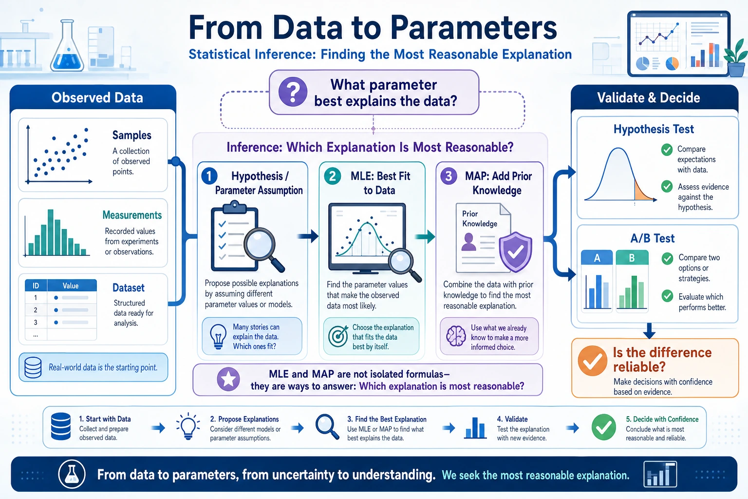
The most important thing in this lesson is not memorizing terminology, but first grasping:

• MLE: which parameters best explain these data?
• MAP: in addition to the data, also consider prior knowledge
• Hypothesis testing: after seeing a difference, how do we judge whether it is just by chance?

Maximum Likelihood Estimation (MLE)

Intuition: Which parameters best explain the data?

You pick up a coin and do not know whether it is fair. You toss it 10 times: HHTHHHTHHH (8 heads, 2 tails).

Question: what is the most likely probability p of landing heads?

Intuition tells you: p ≈ 0.8. MLE turns this intuition into math — find the parameter value that makes the observed data most likely to occur.

A more beginner-friendly analogy

You can first think of MLE as a “detective reconstructing the case” process:

• You have already seen a series of clues (observed data)
• Now you infer backward: which parameter setting looks most like what really happened?

So the core of MLE is not “maximizing for the sake of maximizing,” but:

Find the parameters that best explain the data in front of you.

flowchart LR
    D["Observed data<br/>8 heads, 2 tails"] --> Q["Which p best<br/>explains these data?"]
    Q --> MLE["p = 0.8<br/>(Maximum Likelihood Estimate)"]

    style D fill:#e3f2fd,stroke:#1565c0,color:#333
    style MLE fill:#e8f5e9,stroke:#2e7d32,color:#333

Understanding with code

import numpy as np
import matplotlib.pyplot as plt
from scipy import stats

plt.rcParams['font.sans-serif'] = ['Arial Unicode MS']
plt.rcParams['axes.unicode_minus'] = False

# Observed data: 10 tosses, 8 heads and 2 tails
n_heads = 8
n_tails = 2
n_total = n_heads + n_tails

# For different p values, compute the probability of generating this data (likelihood function)
p_values = np.linspace(0.01, 0.99, 1000)

# Likelihood function: L(p) = C(n,k) * p^k * (1-p)^(n-k)
# We can ignore C(n,k) because it does not depend on p
likelihood = p_values**n_heads * (1 - p_values)**n_tails

# MLE: the p that maximizes the likelihood
p_mle = p_values[np.argmax(likelihood)]
print(f"MLE estimate: p = {p_mle:.3f}")

# Visualization
plt.figure(figsize=(10, 5))
plt.plot(p_values, likelihood, color='steelblue', linewidth=2)
plt.axvline(x=p_mle, color='red', linestyle='--', linewidth=2, label=f'MLE: p = {p_mle:.2f}')
plt.fill_between(p_values, likelihood, alpha=0.1, color='steelblue')
plt.xlabel('p (heads probability)')
plt.ylabel('Likelihood L(p)')
plt.title(f'Likelihood function: tossing a coin 10 times, {n_heads} heads and {n_tails} tails')
plt.legend(fontsize=12)
plt.grid(True, alpha=0.3)
plt.show()

Expected output:

MLE estimate: p = 0.800

Mathematical intuition behind MLE

The answer from MLE is actually very simple: p = number of heads / total number of tosses = 8/10 = 0.8

But the value of MLE is that it is a general framework — for any distribution, you can use the same idea to find the parameters.

Why is this especially important for AI?

Because many loss functions, on the surface, look like they are “doing optimization,” but from a deeper perspective, they are actually:

• finding a set of parameters
• so that those parameters best explain the training data

In other words, MLE is the common language behind many training objectives.

More data = more accurate estimates

# True p = 0.6
rng = np.random.default_rng(seed=42)
true_p = 0.6
n_experiments = [10, 50, 100, 500, 2000]

fig, axes = plt.subplots(1, len(n_experiments), figsize=(20, 4))

for ax, n in zip(axes, n_experiments):
    # Toss the coin n times
    heads = rng.binomial(n, true_p)

    # Likelihood function
    p_vals = np.linspace(0.01, 0.99, 500)
    ll = heads * np.log(p_vals) + (n - heads) * np.log(1 - p_vals)
    ll = np.exp(ll - ll.max())  # Normalize

    p_mle = heads / n
    print(f"n={n:4d}, heads={heads:4d}, MLE={p_mle:.3f}")

    ax.plot(p_vals, ll, color='steelblue', linewidth=2)
    ax.axvline(x=true_p, color='green', linestyle='--', label=f'True p={true_p}')
    ax.axvline(x=p_mle, color='red', linestyle='--', label=f'MLE={p_mle:.3f}')
    ax.set_title(f'n = {n}')
    ax.set_xlabel('p')
    ax.legend(fontsize=8)

plt.suptitle('More data means a more accurate and more certain MLE (the curve becomes narrower)', fontsize=13)
plt.tight_layout()
plt.show()

Expected output with seed=42:

n=  10, heads=   5, MLE=0.500
n=  50, heads=  31, MLE=0.620
n= 100, heads=  69, MLE=0.690
n= 500, heads= 318, MLE=0.636
n=2000, heads=1212, MLE=0.606

Interpretation: The more data you have, the narrower the peak of the likelihood function and the closer it gets to the true value. This is the power of “big data.”

---

Maximum A Posteriori Estimation (MAP)

The problem with MLE

If you only toss a coin 3 times and all three are heads, MLE will tell you p = 3/3 = 1.0 — “this coin always lands heads.”

That is clearly unreasonable. Our common sense tells us that for most coins, p should be close to 0.5.

MAP: adding prior knowledge

MAP adds a “prior” on top of MLE — your prior belief about the parameters:

MAP = likelihood × prior

A better way to remember it

If MLE is:

• only looking at the evidence in front of you

Then MAP is more like:

• the evidence in front of you + your original common sense about the world

So it is very suitable for explaining many phenomena in AI:

• Why adding a constraint to keep parameters from getting too large makes training more stable
• Why regularization is not just a trick, but a kind of prior assumption

# Data: 3 tosses, all heads
n, k = 3, 3

p_values = np.linspace(0.01, 0.99, 1000)

# Likelihood function
likelihood = p_values**k * (1 - p_values)**(n - k)

# Prior: we believe p is likely near 0.5 (represented by a Beta distribution)
prior = stats.beta.pdf(p_values, a=5, b=5)  # Prior centered at 0.5

# Posterior ∝ likelihood × prior
posterior = likelihood * prior
posterior = posterior / np.trapezoid(posterior, p_values)  # Normalize

# Find the maximum
p_mle = p_values[np.argmax(likelihood)]
p_map = p_values[np.argmax(posterior)]

print(f"MLE: p = {p_mle:.3f}")
print(f"MAP: p = {p_map:.3f}")

# Visualization
fig, ax = plt.subplots(figsize=(10, 5))
ax.plot(p_values, likelihood / np.trapezoid(likelihood, p_values),
        '--', color='coral', linewidth=2, label='Likelihood function')
ax.plot(p_values, prior / np.trapezoid(prior, p_values),
        '--', color='green', linewidth=2, label='Prior')
ax.plot(p_values, posterior, color='steelblue', linewidth=2, label='Posterior')
ax.axvline(x=p_mle, color='coral', linestyle=':', alpha=0.7, label=f'MLE = {p_mle:.2f}')
ax.axvline(x=p_map, color='steelblue', linestyle=':', alpha=0.7, label=f'MAP = {p_map:.2f}')
ax.set_xlabel('p')
ax.set_ylabel('Probability density')
ax.set_title('MLE vs MAP (with only 3 data points)')
ax.legend()
ax.grid(True, alpha=0.3)
plt.show()

Expected output:

MLE: p = 0.990
MAP: p = 0.637

Interpretation:

• MLE gives p close to 1.0 (completely biased by very little data)
• MAP gives p≈0.64 (a compromise between data and prior)
• As the amount of data increases, MAP and MLE will converge

MLE vs MAP

	MLE	MAP
Uses prior?	No	Yes
When data is small	Easy to overfit	More stable
When data is large	Approaches MAP	Approaches MLE
Corresponding idea in AI	Ordinary training	Regularization (e.g. L2 regularization = Gaussian prior)

AI connection

L2 regularization (also called weight decay) is essentially MAP — it assumes the prior on weights is a normal distribution with mean 0, encouraging weights not to become too large. This is why regularization helps prevent overfitting.

---

Hypothesis Testing and A/B Testing

A daily-life scenario

You changed the color of a website button (version A uses blue, version B uses green), and version B’s click-through rate increased by 2%.

Question: is this difference real, or just random fluctuation?

The idea behind hypothesis testing

flowchart TD
    A["State the hypothesis"] --> B["H₀: A and B have no difference<br/>(null hypothesis)"]
    A --> C["H₁: B is better than A<br/>(alternative hypothesis)"]
    B --> D["Assume H₀ is true<br/>Calculate how 'unusual'<br/>the observed difference is"]
    D --> E{"p-value < 0.05?"}
    E -->|"Yes"| F["Reject H₀<br/>The difference is significant"]
    E -->|"No"| G["Do not reject H₀<br/>The difference may be random"]

    style F fill:#e8f5e9,stroke:#2e7d32,color:#333
    style G fill:#ffebee,stroke:#c62828,color:#333

Intuition for p-values

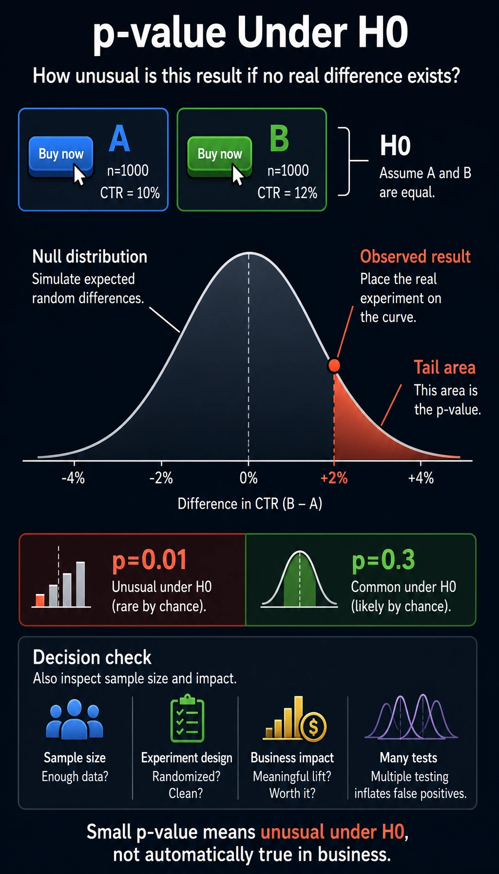
p-value = the probability of getting a difference this large (or larger) just by random fluctuation, assuming there is no real difference.

• Small p-value (for example, 0.01) → “If there were really no difference, this result would almost never happen” → the difference is real
• Large p-value (for example, 0.3) → “Even if there were no real difference, this result would still be common” → it may just be random fluctuation

Be careful with wording: p-value does not prove the alternative hypothesis. It only tells you whether the observed result is unusual under the null hypothesis. In real products, you should also check sample size, experiment design, business impact, and whether you ran many tests at once.

A/B testing in practice

# Simulate an A/B test
rng = np.random.default_rng(seed=2)

# Group A: blue button, true click-through rate 10%
n_a = 1000
clicks_a = rng.binomial(n_a, 0.10)
rate_a = clicks_a / n_a

# Group B: green button, true click-through rate 12% (really better)
n_b = 1000
clicks_b = rng.binomial(n_b, 0.12)
rate_b = clicks_b / n_b

print(f"Group A click-through rate: {rate_a:.1%} ({clicks_a}/{n_a})")
print(f"Group B click-through rate: {rate_b:.1%} ({clicks_b}/{n_b})")
print(f"Difference: {rate_b - rate_a:.1%}")

# Use a z-test
from scipy.stats import norm

# Pooled proportion
p_pool = (clicks_a + clicks_b) / (n_a + n_b)
# Standard error
se = np.sqrt(p_pool * (1 - p_pool) * (1/n_a + 1/n_b))
# z statistic
z = (rate_b - rate_a) / se
# p-value (one-sided)
p_value = 1 - norm.cdf(z)

print(f"\nz statistic: {z:.3f}")
print(f"p-value: {p_value:.4f}")

if p_value < 0.05:
    print("→ p < 0.05, the difference is significant! Version B is indeed better.")
else:
    print("→ p >= 0.05, the difference is not significant and may be due to random fluctuation.")

Expected output with seed=2:

Group A click-through rate: 10.3% (103/1000)
Group B click-through rate: 12.9% (129/1000)
Difference: 2.6%

z statistic: 1.816
p-value: 0.0347
→ p < 0.05, the difference is significant! Version B is indeed better.

Understanding p-values through simulation

# Simulation: if A and B really had no difference (both 10%), how large a difference would we see?
rng = np.random.default_rng(seed=2)
n_simulations = 10000
simulated_diffs = []

for _ in range(n_simulations):
    # Both groups use the same probability of 10%
    sim_a = rng.binomial(1000, 0.10) / 1000
    sim_b = rng.binomial(1000, 0.10) / 1000
    simulated_diffs.append(sim_b - sim_a)

simulated_diffs = np.array(simulated_diffs)

# Plot the distribution
observed_diff = rate_b - rate_a

plt.figure(figsize=(10, 5))
plt.hist(simulated_diffs, bins=50, density=True, color='steelblue',
         edgecolor='white', alpha=0.7, label='Difference distribution under the null hypothesis')
plt.axvline(x=observed_diff, color='red', linewidth=2, linestyle='--',
            label=f'Observed difference: {observed_diff:.3f}')

# p-value = area to the right of the red line
p_sim = (simulated_diffs >= observed_diff).mean()
plt.fill_between(np.linspace(observed_diff, 0.08, 100),
                 0, 30, alpha=0.3, color='red', label=f'p-value ≈ {p_sim:.4f}')

plt.xlabel('Click-through rate difference (B - A)')
plt.ylabel('Density')
plt.title('Intuition for p-values: how "unusual" is the observed difference?')
plt.legend()
plt.grid(True, alpha=0.3)
plt.show()

Add this line if you want a numeric check:

print(f"Simulation p-value: {p_sim:.4f}")

Expected output with seed=2:

Simulation p-value: 0.0262

---

The Connection Between MLE and Loss Functions

MLE = minimizing cross-entropy

This is a very important connection — in classification problems, maximizing likelihood is equivalent to minimizing cross-entropy loss.

# Binary classification problem
# Model prediction: p_hat = the probability the model assigns to label 1
# True label: y ∈ {0, 1}

# Likelihood function
# L = ∏ p_hat^y * (1-p_hat)^(1-y)

# Take logarithm (log-likelihood)
# log L = Σ [y * log(p_hat) + (1-y) * log(1-p_hat)]

# Maximize log L = minimize -log L = minimize cross-entropy!

# Example
y_true = np.array([1, 0, 1, 1, 0])
p_pred = np.array([0.9, 0.2, 0.8, 0.7, 0.3])

# Cross-entropy (manual)
cross_entropy = -np.mean(
    y_true * np.log(p_pred) + (1 - y_true) * np.log(1 - p_pred)
)
print(f"Cross-entropy loss: {cross_entropy:.4f}")

# Log-likelihood (manual)
log_likelihood = np.mean(
    y_true * np.log(p_pred) + (1 - y_true) * np.log(1 - p_pred)
)
print(f"Log-likelihood: {log_likelihood:.4f}")
print(f"Cross-entropy = -log-likelihood: {-log_likelihood:.4f}")

Expected output:

Cross-entropy loss: 0.2530
Log-likelihood: -0.2530
Cross-entropy = -log-likelihood: 0.2530

Why is this important?

When you see nn.CrossEntropyLoss() or nn.BCELoss() in PyTorch, now you know — they are essentially doing maximum likelihood estimation. Loss functions are not defined arbitrarily; they have a deep probabilistic foundation.

---

What should you take into the next section?

After reading this section, the most valuable questions to bring to the next one are:

1. If a model predicts a distribution, how do we measure how different two distributions are?
2. Why can cross-entropy feel both like an information theory concept and a training loss?
3. Why does KL divergence keep showing up in VAE, RLHF, and distillation?

These questions will naturally lead you to:

• 4.2.5 Basics of Information Theory

flowchart LR
    MLE["MLE<br/>Maximum Likelihood Estimation"] --> CE["Cross-entropy loss<br/>Classification tasks"]
    MAP["MAP<br/>Maximum A Posteriori Estimation"] --> REG["Regularization<br/>Prevent overfitting"]

    style MLE fill:#e3f2fd,stroke:#1565c0,color:#333
    style MAP fill:#e3f2fd,stroke:#1565c0,color:#333
    style CE fill:#e8f5e9,stroke:#2e7d32,color:#333
    style REG fill:#e8f5e9,stroke:#2e7d32,color:#333

Connection to later sections

• Next section: Information theory — understand cross-entropy from another perspective
• Station 5: The loss function of logistic regression is cross-entropy (from MLE)
• Station 5: The probabilistic interpretation of regularization (L1/L2) is MAP
• Station 6: Neural network training = minimizing loss functions = doing MLE/MAP

---

Evidence to Keep

Keep this page’s proof of learning as a small evidence card:

Random Process

event, distribution, sample, likelihood, entropy, or Bayes update

Simulation Or Formula

code or formula used to make uncertainty visible

Output

probability, sample statistic, interval, entropy, or updated belief

Failure Check

base-rate confusion, p-value misuse, sample bias, or mixing probability with certainty

Expected Output

numeric result plus interpretation in plain language

Summary

Concept	Intuition	Formula/Code
MLE	Find the parameters that best explain the data	Maximize the likelihood function
MAP	MLE + prior knowledge	Maximize likelihood × prior
p-value	How “unusual” the difference is	The probability of observing such a difference under the null hypothesis
A/B testing	Compare whether two groups have a real difference	scipy.stats
Cross-entropy	Minimizing cross-entropy = MLE	nn.CrossEntropyLoss()

Hands-on Exercises

Exercise 1: Coin Toss MLE

Toss a coin 100 times and get 62 heads.

1. Use MLE to estimate p
2. Plot the likelihood function
3. If the prior is Beta(10, 10), what is the MAP estimate?

Reference implementation:

n = 100
k = 62
p_vals = np.linspace(0.01, 0.99, 1000)

likelihood = p_vals**k * (1 - p_vals)**(n - k)
p_mle = p_vals[np.argmax(likelihood)]

prior = stats.beta.pdf(p_vals, 10, 10)
posterior = likelihood * prior
posterior = posterior / np.trapezoid(posterior, p_vals)
p_map = p_vals[np.argmax(posterior)]

print(f"MLE estimate: {p_mle:.3f}")
print(f"MAP estimate with Beta(10, 10): {p_map:.3f}")

Expected output:

MLE estimate: 0.620
MAP estimate with Beta(10, 10): 0.602

Exercise 2: A/B Testing

Simulate an A/B test: Group A (n=500) has a true conversion rate of 8%, and Group B (n=500) has a true conversion rate of 8% (no difference). Run 1000 experiments and count how many times the p-value is less than 0.05 (this is the “false positive rate,” which should be about 5% in theory).

Reference implementation:

rng = np.random.default_rng(seed=42)
false_positives = 0
n_runs = 1000

for _ in range(n_runs):
    clicks_a = rng.binomial(500, 0.08)
    clicks_b = rng.binomial(500, 0.08)
    rate_a = clicks_a / 500
    rate_b = clicks_b / 500

    p_pool = (clicks_a + clicks_b) / 1000
    se = np.sqrt(p_pool * (1 - p_pool) * (1/500 + 1/500))
    if se == 0:
        continue

    z = (rate_b - rate_a) / se
    p_value = 2 * (1 - norm.cdf(abs(z)))  # two-sided test
    false_positives += p_value < 0.05

print(f"False positive rate: {false_positives / n_runs:.1%} ({false_positives}/{n_runs})")

Expected output with seed=42:

False positive rate: 3.9% (39/1000)

Exercise 3: MLE for a Normal Distribution

Generate 200 samples from N(5, 2), use MLE to estimate the mean and standard deviation (for a normal distribution, the MLE is: mean = sample mean, standard deviation = sample standard deviation), and compare with the true values.

Reference implementation:

rng = np.random.default_rng(seed=42)
samples = rng.normal(5, 2, 200)

mu_hat = samples.mean()
sigma_hat = np.sqrt(((samples - mu_hat) ** 2).mean())

print(f"Estimated mean: {mu_hat:.3f} (true mean: 5)")
print(f"Estimated std: {sigma_hat:.3f} (true std: 2)")

Expected output:

Estimated mean: 4.939 (true mean: 5)
Estimated std: 1.759 (true std: 2)

Operation guide and checkpoints

• For 62 heads in 100 tosses, the MLE is 0.62. With a symmetric Beta(10,10) prior, the MAP estimate moves toward 0.5, about 0.602 in the supplied grid code.
• In the A/B false-positive simulation where both true rates are 8%, the share of p < 0.05 should be around 5%, with random variation. A higher-looking single run is not proof of a real effect.
• The explanation should separate effect size from statistical significance. A p-value answers “how surprising under the null,” not “how important for the business.”