E.C.1 Support Vector Machine

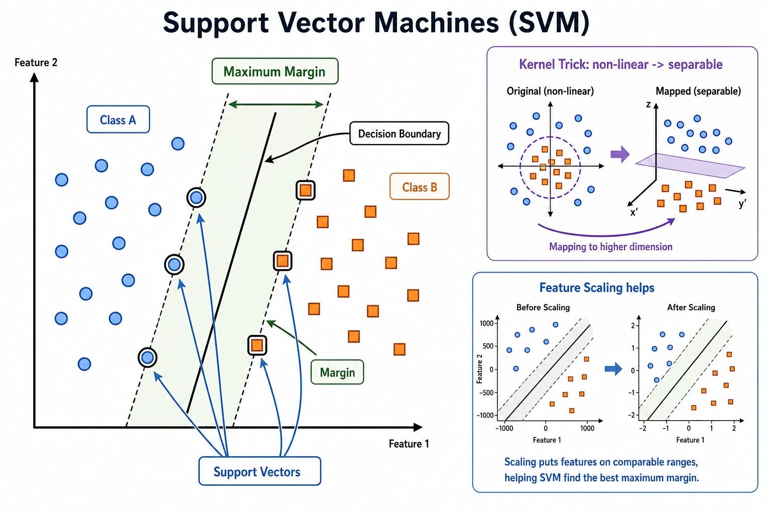
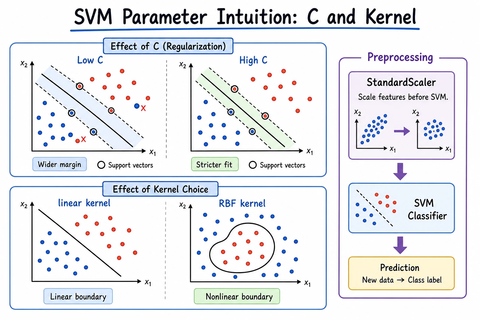
SVM tries to find a decision boundary with a large margin. The points closest to the boundary are the support vectors; they are the samples that most strongly shape the boundary.

What You Need

• Python 3.10+
• Current stable scikit-learn and numpy

python -m pip install -U scikit-learn numpy

Key Terms

• Margin: distance between the boundary and the nearest samples.
• Support vector: a critical sample near the boundary.
• C: controls tolerance for mistakes. Larger C usually fits training data more tightly.
• Kernel: controls whether the boundary is linear or nonlinear.
• Scaling: SVM usually needs normalized feature ranges.

Run A Linear SVM Baseline

Create svm_baseline.py:

import numpy as np
from sklearn.pipeline import make_pipeline
from sklearn.preprocessing import StandardScaler
from sklearn.svm import SVC

X = np.array([
    [1.0, 1.2],
    [1.3, 0.9],
    [1.1, 1.0],
    [4.0, 4.2],
    [4.3, 3.8],
    [3.9, 4.1],
])
y = np.array([0, 0, 0, 1, 1, 1])

model = make_pipeline(
    StandardScaler(),
    SVC(kernel="linear", C=1.0),
)

model.fit(X, y)
pred = model.predict([[1.2, 1.1], [4.2, 4.0]])
svc = model.named_steps["svc"]

print("predictions:", pred.tolist())
print("support_per_class:", svc.n_support_.tolist())

Run it:

python svm_baseline.py

Expected output:

predictions: [0, 1]
support_per_class: [2, 1]

This is the smallest useful SVM habit: scale features, fit the model, predict, then inspect support vectors.

Baseline Review

Review SVM by checking feature scale, boundary shape, and support-vector count. If many samples become support vectors, the boundary may be sensitive to data noise or the classes may not be cleanly separated.

For a project note, include the reason SVM is a fair baseline. Good reasons are small data, meaningful numeric features, and a need for a strong but still interpretable classifier. Weak reasons are “SVM is classic” or “I wanted to try another model.”

Change The Boundary

Run this standalone comparison:

from sklearn.svm import SVC

for kernel in ["linear", "rbf"]:
    if kernel == "linear":
        model = SVC(kernel="linear", C=1.0)
    else:
        model = SVC(kernel="rbf", C=1.0, gamma="scale")
    print(model)

Expected output starts like:

SVC(kernel='linear')
SVC()

Use linear first when the boundary is simple. Try rbf when the boundary is visibly curved or linear SVM underfits.

Practical Rule

Try SVM when:

1. The dataset is small or medium.
2. Features are already meaningful.
3. The class boundary is reasonably clear.
4. You need a strong baseline before heavier models.

Be careful when the dataset is very large or prediction latency must be extremely low.

Evidence to Keep

Keep this page’s proof of learning as a small evidence card:

Model Family

SVM, KNN, Naive Bayes, LDA, or another classical baseline

Dataset View

feature scale, class balance, decision boundary, and train/test split

Metric

accuracy/F1, confusion matrix, margin, neighbor behavior, or projection quality

Failure Check

scaling, high dimensionality, weak assumptions, leakage, or poor baseline fit

Expected Output

classical-ML baseline result with one limitation note

Common Mistakes

• Forgetting StandardScaler().
• Starting with a complex kernel before trying linear.
• Tuning C and kernel before checking feature quality.

Practice

Add two noisy points near the boundary and compare C=0.1, C=1.0, and C=10.0. Record how many support vectors each version uses.

Reference implementation and walkthrough

A good answer records a small table with C, predictions or score, and support-vector count. Lower C usually allows a wider, softer margin and may tolerate noisy points. Higher C tries harder to classify training points correctly, which can make the boundary more sensitive to the new noisy examples.

The exact support-vector counts depend on your added points, so do not fake a universal number. The correct explanation is about the trend and the trade-off between margin softness and fitting noisy training cases.