4.3.5 Chain Rule and Backpropagation Preview

This section is the bridge between mathematics and deep learning

The chain rule explains a core question: For a neural network with hundreds of layers, how do we compute the derivative of the loss function with respect to each parameter? The answer is backpropagation — in essence, it is the systematic application of the chain rule.

Learning Objectives

• Understand the chain rule — how to differentiate composite functions
• Manually derive backpropagation for a simple two-layer network
• Understand computation graphs — why PyTorch needs them
• Get ready for deep learning in Station 6

First, set a very important learning expectation

This section is one of the easiest places in Station 4 to make newcomers feel overwhelmed. So what you should focus on first in this section is not every formula, but:

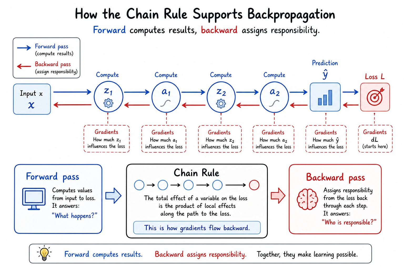
• A complex network is still just many simple steps linked together
• Backpropagation is not a mysterious algorithm; it is the chain rule applied layer by layer
• PyTorch’s backward() is essentially helping you do this automatically

---

First, build a map

This lesson is the bridge from Station 4 to deep learning in Station 6.

If what you learned before was:

• Derivatives: how one quantity changes
• Gradients: how many quantities change together
• Gradient descent: how to update parameters

Then what this lesson adds is:

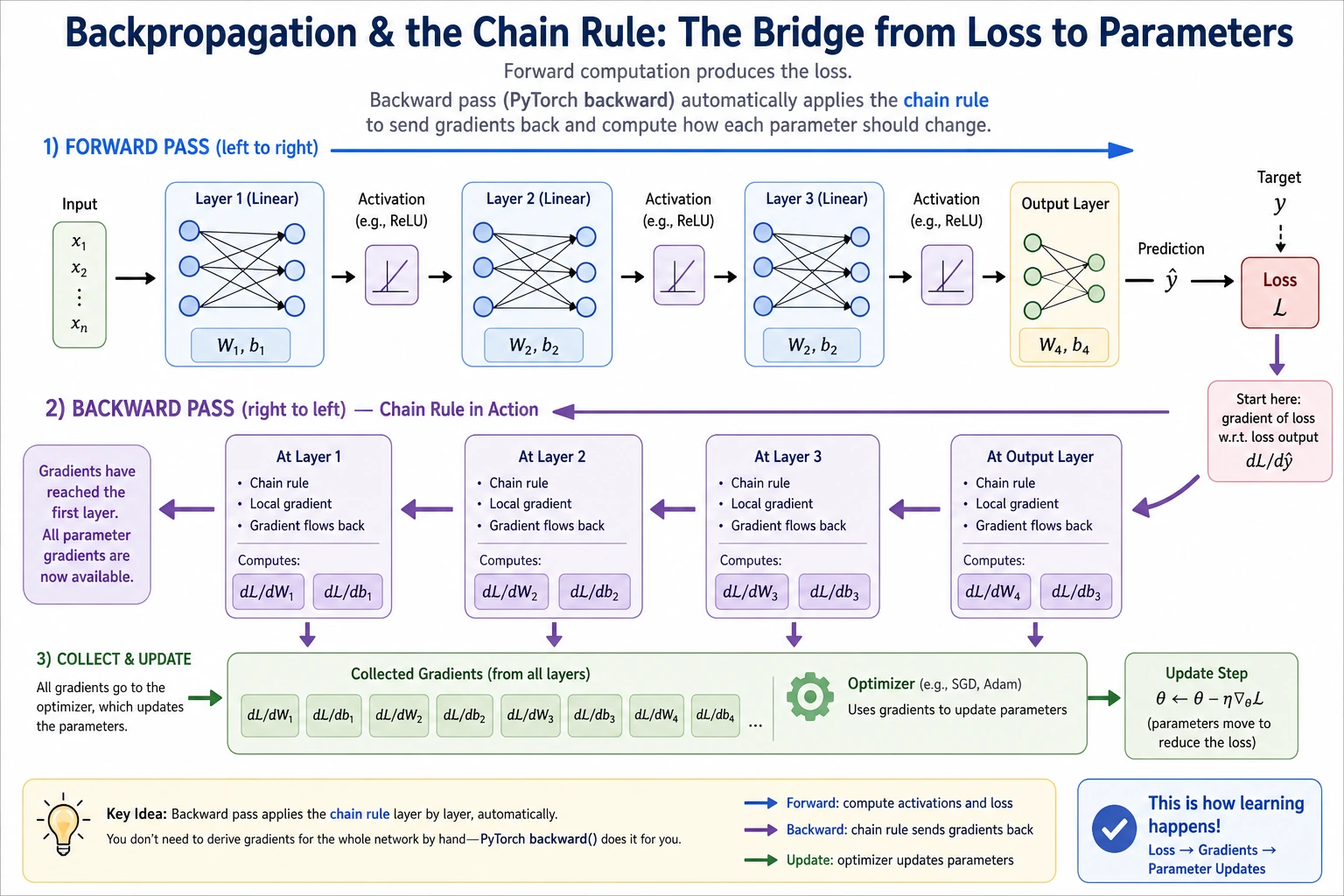
• In a many-layer network, how the gradient is actually computed layer by layer

The Chain Rule — the “Peel the Onion” Method

Intuition

If a function has a nested structure — one function wrapped inside another — then its derivative is found by peeling it layer by layer and multiplying the derivatives at each layer.

flowchart LR
    X["x"] -->|"g(x)"| U["u = g(x)"]
    U -->|"f(u)"| Y["y = f(g(x))"]

    style X fill:#e3f2fd,stroke:#1565c0,color:#333
    style U fill:#fff3e0,stroke:#e65100,color:#333
    style Y fill:#e8f5e9,stroke:#2e7d32,color:#333

Chain rule: dy/dx = (dy/du) × (du/dx)

“The rate of change of y with respect to x = the rate of change of y with respect to u × the rate of change of u with respect to x”

A more beginner-friendly analogy

You can first think of the chain rule as a row of gears:

• The first gear turns a little
• It causes the second gear to turn
• The second gear then drives the third

So how the last quantity changes depends on the multiplier for “passing along change” at each intermediate layer.

That is why the core action of the chain rule is:

• Break the function apart layer by layer
• Multiply the rates of change layer by layer

Everyday intuition

If your salary increases by 10% and prices increase by 5%, how does your real purchasing power change?

• Salary change → affects your wallet → affects purchasing power
• Total change = salary change rate × conversion rate

Multiply the change rates of each step = the overall change rate.

Calculation Example

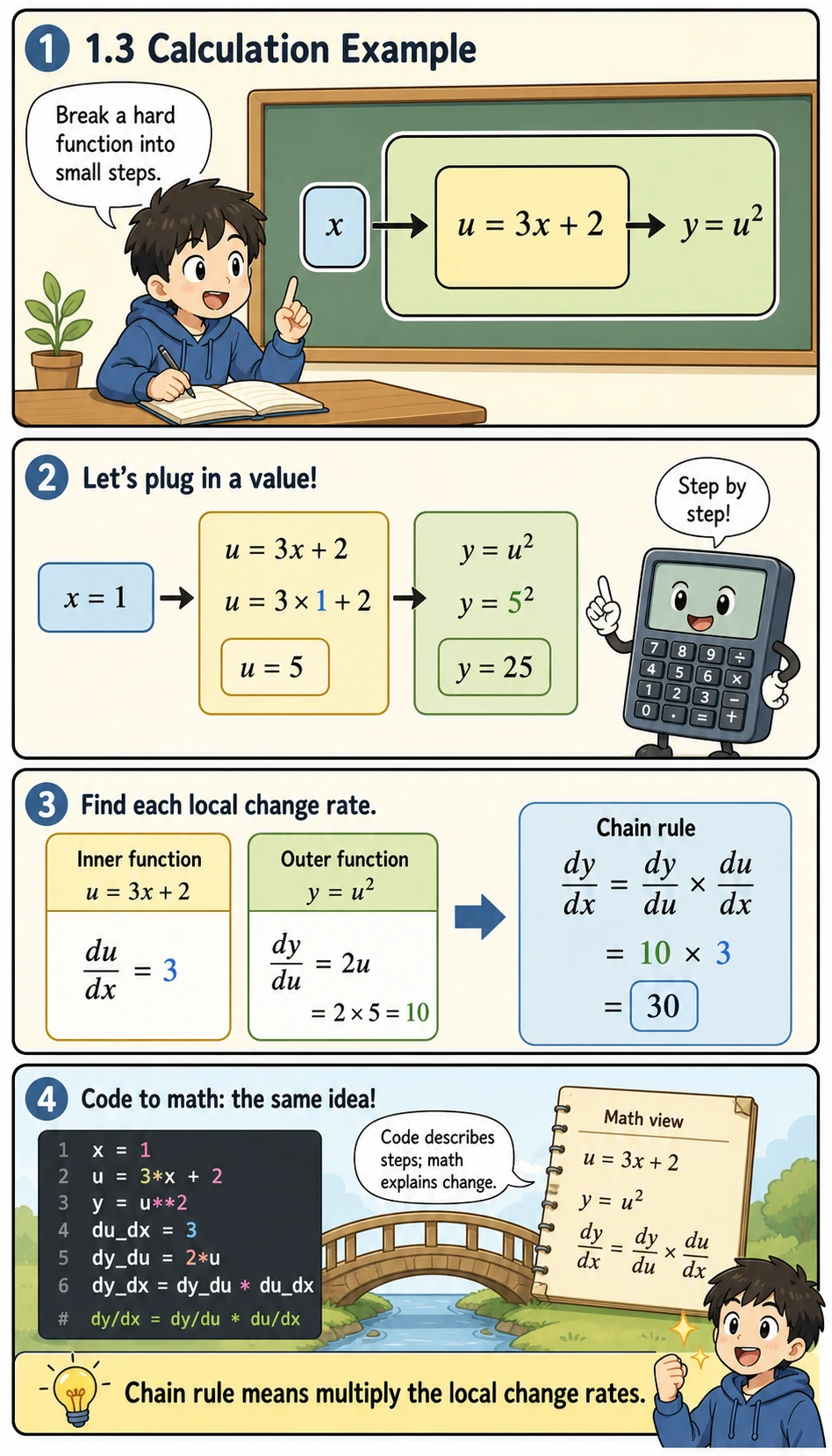
Before looking at the code, read this example as a small assembly line:

• u = 3x + 2 is the inner step, so it tells us how u changes when x changes
• y = u² is the outer step, so it tells us how y changes when u changes
• dy_dx means “how much the final output y changes if the original input x changes a little”
• numerical_derivative is a safety check: it estimates the slope by moving x a tiny bit left and right

So the code below is not just computing an answer. It is showing the same idea three ways: decomposition, formula, and numerical verification.

import numpy as np

# Example: y = (3x + 2)²
# Decomposition: u = 3x + 2, y = u²
# dy/dx = dy/du × du/dx = 2u × 3 = 6(3x + 2)

# Method 1: Chain rule
def chain_rule_example(x):
    u = 3 * x + 2        # inner function
    y = u ** 2            # outer function

    du_dx = 3             # derivative of inner function
    dy_du = 2 * u         # derivative of outer function
    dy_dx = dy_du * du_dx # chain rule

    return y, dy_dx

# Method 2: numerical check
def numerical_derivative(f, x, h=1e-7):
    return (f(x + h) - f(x - h)) / (2 * h)

f = lambda x: (3*x + 2)**2

x0 = 1
y, dy_dx_chain = chain_rule_example(x0)
dy_dx_numerical = numerical_derivative(f, x0)

print(f"x = {x0}")
print(f"  Chain rule: dy/dx = {dy_dx_chain}")
print(f"  Numerical check: dy/dx = {dy_dx_numerical:.4f}")

Multi-layer chain rule

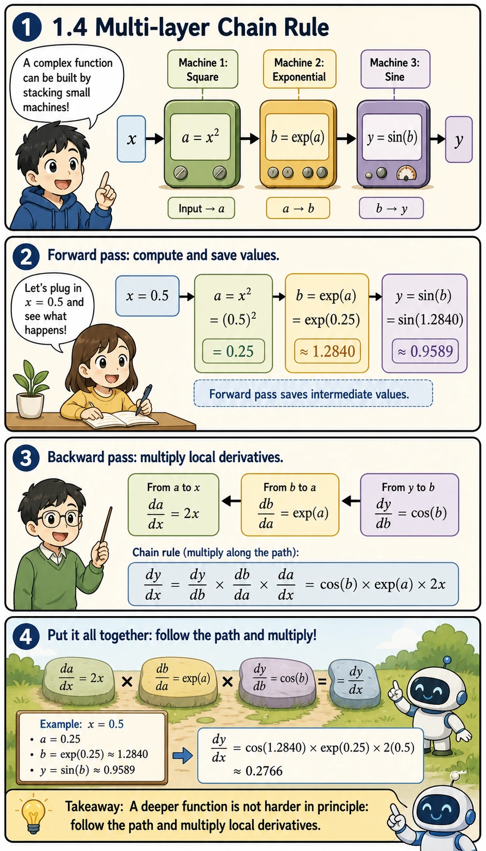
What if there are even more nested layers? The same idea still works, layer by layer:

• First compute forward values: a, then b, then y
• Then compute local derivatives: da_dx, db_da, and dy_db
• Finally multiply the derivatives along the path from output back to input

This is the exact mental model you will reuse in neural networks: a deep model is a longer path, not a completely different kind of math.

# y = sin(exp(x²))
# Decomposition: a = x², b = exp(a), y = sin(b)
# dy/dx = dy/db × db/da × da/dx
#       = cos(b) × exp(a) × 2x

x0 = 0.5
a = x0 ** 2
b = np.exp(a)
y = np.sin(b)

da_dx = 2 * x0
db_da = np.exp(a)
dy_db = np.cos(b)

dy_dx = dy_db * db_da * da_dx

# Numerical check
f = lambda x: np.sin(np.exp(x**2))
dy_dx_num = numerical_derivative(f, x0)

print(f"Chain rule: {dy_dx:.6f}")
print(f"Numerical check: {dy_dx_num:.6f}")

---

Backpropagation — a Systematic Use of the Chain Rule

A Two-Layer Neural Network

flowchart LR
    X["Input x"] --> H["Hidden layer<br/>h = relu(w1·x + b1)"]
    H --> O["Output layer<br/>y = w2·h + b2"]
    O --> L["Loss<br/>L = (y - target)²"]

    style X fill:#e3f2fd,stroke:#1565c0,color:#333
    style H fill:#fff3e0,stroke:#e65100,color:#333
    style O fill:#fff3e0,stroke:#e65100,color:#333
    style L fill:#ffebee,stroke:#c62828,color:#333

Forward Pass

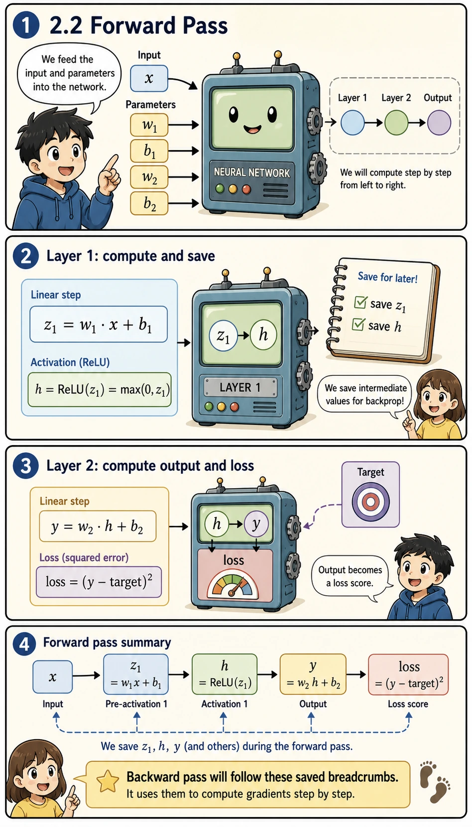
Forward pass means “compute from input to prediction to loss.” In this tiny network, the important point is not the size of the model, but the habit of saving intermediate values:

• z1 is the result before the activation function
• h is the hidden representation after ReLU
• y is the prediction
• loss measures how wrong the prediction is

These values become the breadcrumbs used by the backward pass.

# Input and target
x = 2.0
target = 1.0

# Parameters
w1 = 0.5
b1 = 0.1
w2 = -0.3
b2 = 0.2

# --- Forward pass ---
# Layer 1: linear + ReLU
z1 = w1 * x + b1
h = max(0, z1)       # ReLU

# Layer 2: linear
y = w2 * h + b2

# Loss
loss = (y - target) ** 2

print("=== Forward Pass ===")
print(f"z1 = w1*x + b1 = {w1}*{x} + {b1} = {z1}")
print(f"h  = ReLU(z1) = {h}")
print(f"y  = w2*h + b2 = {w2}*{h} + {b2} = {y}")
print(f"loss = (y - target)² = ({y} - {target})² = {loss:.4f}")

Why must we always compute the forward pass before the backward pass?

Because backpropagation does not happen out of thin air. It must be based on the intermediate values already computed during the forward pass:

• z1
• h
• y
• loss

So a very stable way to understand it is:

• The forward pass lays out the path
• The backward pass follows this path and sends gradients back layer by layer

Backward Pass

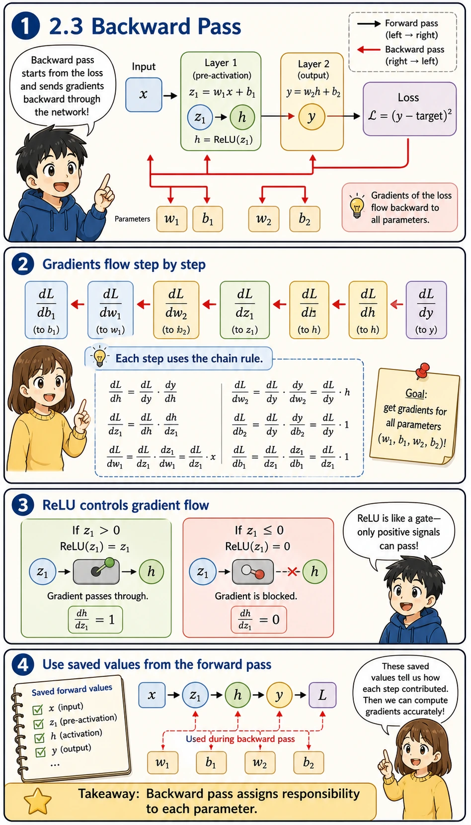
Starting from the loss, compute the gradient of each parameter layer by layer:

Read symbols like dL_dw1 as “how sensitive the loss L is to parameter w1.” If the absolute value is large, changing that parameter has a large effect on the loss. If it is close to zero, that parameter currently has little influence.

The backward pass is therefore a responsibility assignment process:

• Start with the loss
• Ask how the loss depends on the output
• Ask how the output depends on each earlier value
• Keep multiplying local derivatives until every parameter gets its gradient

The ReLU gate is especially important: if z1 <= 0, the gradient through that path becomes 0.

# --- Backward pass ---
# Start from the last layer and work backward using the chain rule

# dL/dy
dL_dy = 2 * (y - target)
print(f"\n=== Backward Pass ===")
print(f"dL/dy = 2*(y-target) = {dL_dy:.4f}")

# dL/dw2 = dL/dy × dy/dw2 = dL/dy × h
dL_dw2 = dL_dy * h
print(f"dL/dw2 = dL/dy × h = {dL_dy:.4f} × {h} = {dL_dw2:.4f}")

# dL/db2 = dL/dy × dy/db2 = dL/dy × 1
dL_db2 = dL_dy * 1
print(f"dL/db2 = dL/dy × 1 = {dL_db2:.4f}")

# dL/dh = dL/dy × dy/dh = dL/dy × w2
dL_dh = dL_dy * w2
print(f"dL/dh  = dL/dy × w2 = {dL_dy:.4f} × {w2} = {dL_dh:.4f}")

# dL/dz1 = dL/dh × dh/dz1 (ReLU derivative: 1 when z1 > 0, otherwise 0)
relu_grad = 1.0 if z1 > 0 else 0.0
dL_dz1 = dL_dh * relu_grad
print(f"dL/dz1 = dL/dh × relu'(z1) = {dL_dh:.4f} × {relu_grad} = {dL_dz1:.4f}")

# dL/dw1 = dL/dz1 × dz1/dw1 = dL/dz1 × x
dL_dw1 = dL_dz1 * x
print(f"dL/dw1 = dL/dz1 × x = {dL_dz1:.4f} × {x} = {dL_dw1:.4f}")

# dL/db1 = dL/dz1 × dz1/db1 = dL/dz1 × 1
dL_db1 = dL_dz1 * 1
print(f"dL/db1 = dL/dz1 × 1 = {dL_db1:.4f}")

Update Parameters with the Gradients

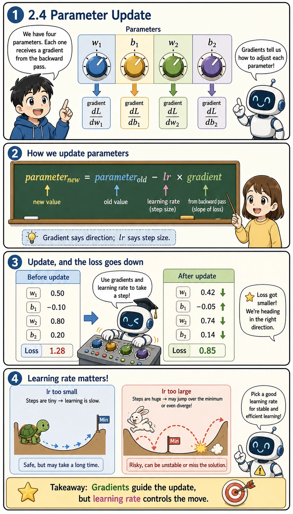
After backpropagation, gradients are not the final goal. They are instructions for how to update the parameters.

The update rule is:

new parameter = old parameter - learning rate × gradient

lr means learning rate. It controls how large each update step is. A very small lr learns slowly; a very large lr may jump past the good region and make the loss worse.

lr = 0.1

print(f"\n=== Parameter Update (lr={lr}) ===")
print(f"w1: {w1:.4f} → {w1 - lr * dL_dw1:.4f}")
print(f"b1: {b1:.4f} → {b1 - lr * dL_db1:.4f}")
print(f"w2: {w2:.4f} → {w2 - lr * dL_dw2:.4f}")
print(f"b2: {b2:.4f} → {b2 - lr * dL_db2:.4f}")

# Update
w1 -= lr * dL_dw1
b1 -= lr * dL_db1
w2 -= lr * dL_dw2
b2 -= lr * dL_db2

# Check whether the loss decreased
z1_new = w1 * x + b1
h_new = max(0, z1_new)
y_new = w2 * h_new + b2
loss_new = (y_new - target) ** 2

print(f"\nLoss change: {loss:.4f} → {loss_new:.4f} ({'↓ decreased!' if loss_new < loss else '↑ increased'})")

---

Computation Graphs — the Data Structure Behind Backpropagation

What Is a Computation Graph?

Computation graph = a directed graph that represents each operation as a node.

flowchart LR
    x["x = 2"] --> mul1["× w1"]
    w1["w1 = 0.5"] --> mul1
    mul1 --> add1["+ b1"]
    b1["b1 = 0.1"] --> add1
    add1 --> relu["ReLU"]
    relu --> mul2["× w2"]
    w2["w2 = -0.3"] --> mul2
    mul2 --> add2["+ b2"]
    b2["b2 = 0.2"] --> add2
    add2 --> sub["- target"]
    sub --> sq["²"]
    sq --> L["Loss"]

    style x fill:#e3f2fd,stroke:#1565c0,color:#333
    style L fill:#ffebee,stroke:#c62828,color:#333

Forward pass: compute in the direction of the arrows, from input to loss.

Backward pass: go against the arrows, from the loss back to each parameter’s gradient.

Why does a computation graph suddenly make everything clear?

Because it reduces a “complex network” into many small nodes:

• Multiplication
• Addition
• Activation
• Loss

Once you see the network as a graph made of these connected nodes, backpropagation no longer feels like magic, but more like:

• Sending gradients back along the graph layer by layer

Why Does PyTorch Need a Computation Graph?

# In PyTorch (we will study this in detail in Station 6)
# import torch
#
# x = torch.tensor(2.0)
# w1 = torch.tensor(0.5, requires_grad=True)
# b1 = torch.tensor(0.1, requires_grad=True)
# w2 = torch.tensor(-0.3, requires_grad=True)
# b2 = torch.tensor(0.2, requires_grad=True)
#
# # Forward pass (PyTorch automatically builds the computation graph)
# h = torch.relu(w1 * x + b1)
# y = w2 * h + b2
# loss = (y - 1.0) ** 2
#
# # Backward pass (one line of code, all gradients computed automatically!)
# loss.backward()
#
# print(w1.grad)  # dL/dw1
# print(b1.grad)  # dL/db1
# print(w2.grad)  # dL/dw2
# print(b2.grad)  # dL/db2

During the forward pass, PyTorch automatically records each operation it performs (building the computation graph), and then loss.backward() propagates backward along the graph, using the chain rule to compute the gradient of each parameter automatically.

Why is this so powerful?

Manually computing the gradients of 4 parameters is already tedious. GPT-3 has 175 billion parameters — manual calculation would be impossible. PyTorch’s automatic differentiation engine (autograd) lets you write only the forward pass code, while gradient computation is fully automated.

---

Full Example: Training a Small Network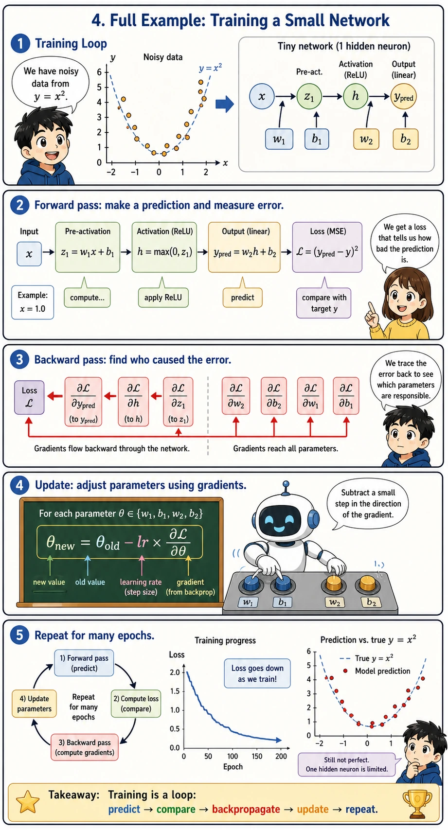

Put the forward pass + backward pass + parameter update together to train a two-layer network:

This complete example is the smallest version of an AI training loop:

1. Read one data point
2. Run the forward pass to make a prediction
3. Compute the loss
4. Run the backward pass to compute gradients
5. Update parameters and repeat for many epochs

An epoch means one full pass over the training data. The list losses records whether training is generally moving in the right direction.

import numpy as np
import matplotlib.pyplot as plt

# Data
rng = np.random.default_rng(seed=42)
X_data = rng.uniform(-2, 2, 50)
y_data = X_data ** 2 + rng.normal(size=50) * 0.3  # y = x² + noise

# Two-layer network parameters
w1 = rng.normal()
b1 = 0.0
w2 = rng.normal()
b2 = 0.0

lr = 0.01
losses = []

for epoch in range(500):
    total_loss = 0

    for x, target in zip(X_data, y_data):
        # === Forward pass ===
        z1 = w1 * x + b1
        h = max(0, z1)
        y_pred = w2 * h + b2
        loss = (y_pred - target) ** 2
        total_loss += loss

        # === Backward pass ===
        dL_dy = 2 * (y_pred - target)
        dL_dw2 = dL_dy * h
        dL_db2 = dL_dy
        dL_dh = dL_dy * w2
        dL_dz1 = dL_dh * (1.0 if z1 > 0 else 0.0)
        dL_dw1 = dL_dz1 * x
        dL_db1 = dL_dz1

        # === Update parameters ===
        w1 -= lr * dL_dw1
        b1 -= lr * dL_db1
        w2 -= lr * dL_dw2
        b2 -= lr * dL_db2

    losses.append(total_loss / len(X_data))
    if epoch % 100 == 0:
        print(f"Epoch {epoch}: loss = {losses[-1]:.4f}")

# Visualization
fig, axes = plt.subplots(1, 2, figsize=(14, 5))

axes[0].plot(losses, color='coral', linewidth=2)
axes[0].set_xlabel('Epoch')
axes[0].set_ylabel('Loss')
axes[0].set_title('Training Loss')
axes[0].grid(True, alpha=0.3)

x_test = np.linspace(-2, 2, 200)
y_pred_test = []
for x in x_test:
    z1 = w1 * x + b1
    h = max(0, z1)
    y_pred_test.append(w2 * h + b2)

axes[1].scatter(X_data, y_data, alpha=0.4, s=20, color='gray', label='Data')
axes[1].plot(x_test, x_test**2, 'g--', linewidth=2, label='y = x² (true)')
axes[1].plot(x_test, y_pred_test, 'r-', linewidth=2, label='Network prediction')
axes[1].set_title('Fit result (two-layer network, 1 hidden neuron)')
axes[1].legend()
axes[1].grid(True, alpha=0.3)

plt.tight_layout()
plt.show()

Limitation of using only 1 neuron

This network has only 1 hidden neuron (essentially a piecewise linear function), so it is not enough to perfectly fit x². Adding more neurons can fit it better — this is what you will learn in Station 6.

---

Evidence to Keep

Keep this page’s proof of learning as a small evidence card:

Function

objective, loss, derivative, gradient, or chain-rule expression

Calculation

numeric derivative, gradient step, or backprop trace

Output

slope, gradient vector, updated parameter, or loss change

Failure Check

sign error, learning rate too large, local slope misunderstanding, or broken chain

Expected Output

calculation trace showing how a parameter changes

Summary

Concept	Intuition
Chain rule	The derivative of a composite function = the product of derivatives at each layer
Forward pass	Compute step by step from input to loss
Backward pass	Compute gradients step by step from loss back to parameters
Computation graph	Records the operations and supports automatic differentiation
Automatic differentiation	PyTorch automatically computes all gradients for you

What should you take away from this lesson?

• The most important intuition of the chain rule is that “changes pass through multiple layers step by step”
• The most important intuition of backpropagation is that “starting from the loss, gradients are passed back layer by layer”
• The most important value of a computation graph is that it turns this into a process that can be recorded and automated

flowchart LR
    FW["Forward pass<br/>Input → Loss"] --> BW["Backward pass<br/>Loss → Gradients"]
    BW --> UP["Parameter update<br/>Gradient descent"]
    UP --> FW

    style FW fill:#e3f2fd,stroke:#1565c0,color:#333
    style BW fill:#ffebee,stroke:#c62828,color:#333
    style UP fill:#e8f5e9,stroke:#2e7d32,color:#333

Chapter Review & Stage Summary

In the three calculus lessons + this lesson, you learned:

1. Derivatives: the speed of change, and the direction for optimization
2. Partial derivatives and gradients: the direction in a multivariable setting, pointing toward the steepest ascent
3. Gradient descent: the core of AI training — taking steps along the negative gradient
4. Chain rule and backpropagation: efficiently computing the gradient of each parameter

🔖 Station 4 complete!

You now have mastered the three major mathematical foundations needed for AI:

• Linear algebra: vectors, matrices, eigenvalues — data representation and transformation
• Probability and statistics: probability distributions, Bayes, MLE — uncertainty and loss functions
• Calculus: derivatives, gradients, gradient descent — how models learn

🔀 Next step: move on to Station 5 · Machine Learning and apply these mathematical tools to practical machine learning algorithms.

---

Hands-On Exercises

Exercise 1: Manual Chain Rule

For y = (2x + 1)³, use the chain rule to find dy/dx, and verify it at x = 1.

Exercise 2: Extend the Network

Change the two-layer network in Section 4 to have 3 hidden neurons (w1 becomes 3 weights), and manually write out the forward pass and backward pass code.

Exercise 3: Compare Manual vs. Automatic

If you have PyTorch installed, use torch.autograd to compute the gradients of all parameters in Section 2, and compare them with your manual results.

If import torch fails, install PyTorch first. For a simple CPU or macOS setup, this usually works:

python -m pip install --upgrade torch

import torch

x = torch.tensor(2.0)
w1 = torch.tensor(0.5, requires_grad=True)
b1 = torch.tensor(0.1, requires_grad=True)
w2 = torch.tensor(-0.3, requires_grad=True)
b2 = torch.tensor(0.2, requires_grad=True)

h = torch.relu(w1 * x + b1)
y = w2 * h + b2
loss = (y - 1.0) ** 2
loss.backward()

print("loss =", loss.item())
print("w1.grad =", w1.grad.item())
print("b1.grad =", b1.grad.item())
print("w2.grad =", w2.grad.item())
print("b2.grad =", b2.grad.item())

Operation guide and checkpoints

• For y=(2x+1)^3, the derivative is 6(2x+1)^2; at x=1, the value is 54.
• When extending the network to 3 hidden neurons, write the hidden layer as a vector and keep gradients for each weight separate. The main check is that every forward value has a corresponding backward gradient.
• Autograd and manual gradients should match up to rounding. If they differ, check ReLU’s active/inactive branch, missing chain-rule factors, and whether the same loss definition was used.