6.3.3 Basic CNN Architecture

Learning Objectives

Describe the path image -> conv block -> feature map -> classifier head -> logits.
Explain why channels usually increase while height and width decrease.
Run a small convolution block and read its output shape.
Build a complete TinyCNN in PyTorch.
Compare Flatten and Global Average Pooling (GAP) from an engineering point of view.

Start with the Whole Pipeline

CNN feature map pipeline

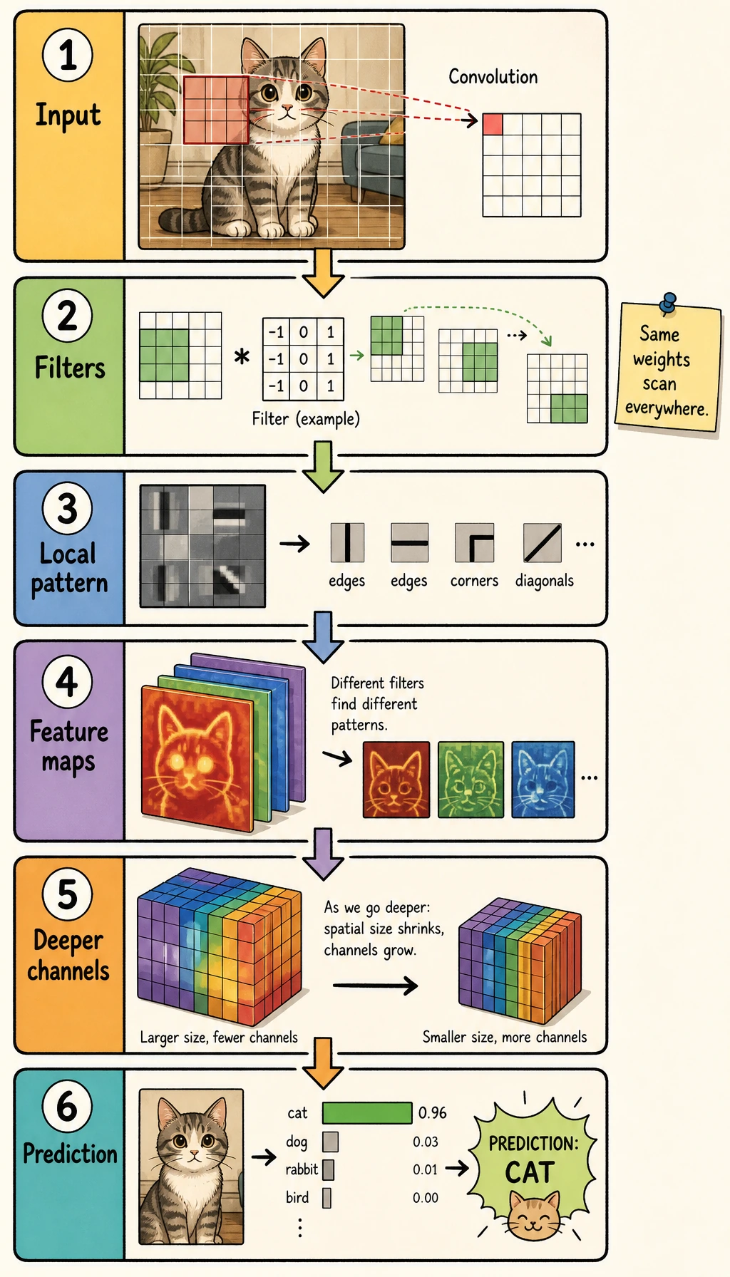
Read the picture from left to right:

imagelow-level featurescompressed feature mapsclassifier headclass scores

A CNN is usually split into two parts:

Part	Job	Typical layers
feature extractor	turn pixels into useful feature maps	`Conv2d`, `ReLU`, `BatchNorm2d`, `MaxPool2d`
classifier head	turn final feature maps into class scores	`Flatten` or GAP, `Linear`

The output of the final layer is usually called logits: raw class scores before softmax.

Channels Go Up, Spatial Size Goes Down

CNN channel count vs spatial size trade-off

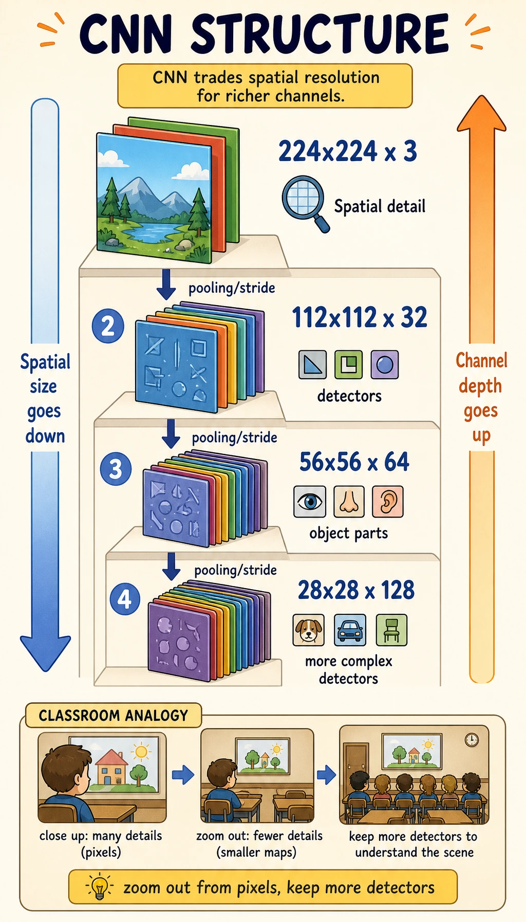
Early layers keep more spatial detail. Deeper layers keep fewer pixels but more feature types.

Stage	Shape intuition	Meaning
input	`[N, 3, 32, 32]`	RGB images
early feature	`[N, 16, 32, 32]`	many edge and texture detectors
after pooling	`[N, 16, 16, 16]`	smaller map, strongest local signals kept
deeper feature	`[N, 64, 8, 8]`	more abstract patterns

This tradeoff is the heart of CNN design:

fewer spatial positions reduces compute;
more channels let the model store richer visual evidence;
the classifier head should see enough semantics, not every raw pixel.

Lab 1: MaxPool by Hand

MaxPool2d(2) keeps the strongest value in each 2 x 2 window.

import numpy as np

feature_map = np.array(
    [
        [1, 3, 2, 0],
        [4, 6, 1, 2],
        [0, 1, 5, 3],
        [2, 4, 1, 7],
    ],
    dtype=np.float32,
)

pooled = np.array(
    [
        [feature_map[0:2, 0:2].max(), feature_map[0:2, 2:4].max()],
        [feature_map[2:4, 0:2].max(), feature_map[2:4, 2:4].max()],
    ]
)

print("maxpool_lab")
print(pooled)

Expected output:

maxpool_lab
[[6. 2.]
 [4. 7.]]

Pooling loses some detail, but it keeps the strongest local response. For classification, that is often a useful bias: the model cares more that a feature appeared than the exact pixel where it appeared.

Lab 2: Run One Convolution Block

A basic CNN block is:

Conv2dactivationoptional pooling

Run it:

import torch
from torch import nn

block = nn.Sequential(
    nn.Conv2d(3, 8, kernel_size=3, padding=1),
    nn.ReLU(),
    nn.MaxPool2d(kernel_size=2),
)

x = torch.randn(2, 3, 32, 32)
y = block(x)

print("block_lab")
print("input:", tuple(x.shape))
print("output:", tuple(y.shape))

Expected output:

block_lab
input: (2, 3, 32, 32)
output: (2, 8, 16, 16)

What changed:

batch stays 2;
channels change from 3 to 8;
height and width shrink from 32 to 16 because of MaxPool2d(2).

In production CNNs, you often see this variant:

Conv2dBatchNorm2dReLU

BatchNorm2d stabilizes feature scale during training. It is useful, but the first model should be kept simple until the shape flow is clear.

Lab 3: Build a Complete Tiny CNN

This model accepts grayscale 28 x 28 images and returns 10 class scores.

import torch
from torch import nn


class TinyCNN(nn.Module):
    def __init__(self, num_classes=10):
        super().__init__()
        self.conv1 = nn.Conv2d(1, 8, kernel_size=3, padding=1)
        self.pool1 = nn.MaxPool2d(2)
        self.conv2 = nn.Conv2d(8, 16, kernel_size=3, padding=1)
        self.pool2 = nn.MaxPool2d(2)
        self.classifier = nn.Sequential(
            nn.Flatten(),
            nn.Linear(16 * 7 * 7, 64),
            nn.ReLU(),
            nn.Linear(64, num_classes),
        )

    def forward(self, x):
        print("shape_trace")
        print(f"{'input':<8} {tuple(x.shape)}")
        x = torch.relu(self.conv1(x))
        print(f"{'conv1':<8} {tuple(x.shape)}")
        x = self.pool1(x)
        print(f"{'pool1':<8} {tuple(x.shape)}")
        x = torch.relu(self.conv2(x))
        print(f"{'conv2':<8} {tuple(x.shape)}")
        x = self.pool2(x)
        print(f"{'pool2':<8} {tuple(x.shape)}")
        x = self.classifier(x)
        print(f"{'logits':<8} {tuple(x.shape)}")
        return x


model = TinyCNN(num_classes=10)
x = torch.randn(4, 1, 28, 28)
_ = model(x)

Expected output:

shape_trace
input    (4, 1, 28, 28)
conv1    (4, 8, 28, 28)
pool1    (4, 8, 14, 14)
conv2    (4, 16, 14, 14)
pool2    (4, 16, 7, 7)
logits   (4, 10)

The final shape is [4, 10] because there are four images and ten scores per image.

Read the Architecture Like an Engineer

When you inspect a CNN, do not only read layer names. Track the tensor contract at every boundary.

Line	Contract to check
`Conv2d(1, 8, ...)`	input must have one channel
`MaxPool2d(2)`	height and width are divided by two
`Conv2d(8, 16, ...)`	previous output channels must be eight
`Linear(16 * 7 * 7, 64)`	flattened feature size must match the actual feature map
final `Linear(..., 10)`	output dimension must equal number of classes

Most CNN bugs are contract bugs: the tensor shape reaching a layer is different from what that layer expects.

Flatten vs Global Average Pooling

Flatten turns all spatial positions into one long vector:

[N, 16, 7, 7] -> [N, 784]

GAP keeps one average value per channel:

[N, 16, 7, 7] -> [N, 16]

Compare parameter counts:

from torch import nn


def count_params(module):
    return sum(p.numel() for p in module.parameters() if p.requires_grad)


flatten_head = nn.Linear(16 * 7 * 7, 10)
gap_head = nn.Linear(16, 10)

print("head_param_lab")
print("flatten head:", count_params(flatten_head))
print("gap head    :", count_params(gap_head))

Expected output:

head_param_lab
flatten head: 7850
gap head    : 170

Use the tradeoff like this:

Head	Strength	Cost
Flatten + Linear	simple, can use location-specific details	many parameters, fixed input size
GAP + Linear	compact, works with variable spatial size more easily	may discard fine location detail

Modern CNN classifiers often use GAP because it reduces overfitting risk and makes the head smaller.

Evidence to Keep

Keep one CNN shape trace:

Input: [batch, channels, height, width]
After Conv: channels change, spatial size follows padding/stride
After Pool: height and width shrink
Before Head: flattened size or GAP output is known
Logits: [batch, num_classes]
Head Choice: Flatten for location-specific detail, GAP for compact classifier

Common Mistakes

Mistake	Symptom	Fix
wrong channel order	`expected input ... to have C channels`	use `[N, C, H, W]` in PyTorch
wrong `Linear` input size	matrix multiplication shape error	print shape before `Flatten`
too much pooling too early	feature maps become tiny	trace `H` and `W` after every block
treating logits as probabilities	confusing loss or evaluation	use logits with `CrossEntropyLoss`; apply `softmax` only for display
adding BatchNorm without understanding mode	train/eval behavior differs	call `model.train()` for training and `model.eval()` for evaluation

Exercises

Change conv2 from 16 output channels to 32. Which lines must change?
Replace the classifier with AdaptiveAvgPool2d((1, 1)), Flatten, and Linear(16, 10).
Remove one pooling layer and predict the new flattened size before running the code.
Add a BatchNorm2d(8) after conv1; verify that the shape stays unchanged.
Write down the shape after every line for an RGB 64 x 64 input.

Reference implementation and walkthrough

If conv2 outputs 32 channels, later layers that expect 16 channels must change too, especially the classifier input size or any next convolution.
With AdaptiveAvgPool2d((1, 1)), the classifier receives one value per channel. If the last feature map has 16 channels, Linear(16, 10) is the right head.
Removing pooling keeps spatial dimensions larger, so the flattened vector grows. Predicting this before running is the main shape-debugging skill.
BatchNorm2d(8) normalizes the 8 channels from conv1; it does not change batch, channel count, height, or width.
For RGB input, the first channel dimension is 3. After that, each convolution changes channels and each pooling/stride changes spatial size. A line-by-line shape trace should make every classifier dimension explainable.

Key Takeaways

A CNN is a feature extractor plus a classifier head.
Convolution blocks increase feature channels; pooling or stride usually reduces spatial size.
Shape tracing is the fastest way to debug CNN architecture.
Flatten is simple but parameter-heavy; GAP is compact and common in modern CNNs.
A strong CNN design is mostly about controlling information flow, not stacking layers blindly.