4.3.4 Gradient Descent: The Most Core Optimization Algorithm in AI

This section is the climax of the entire math phase

Gradient descent is the foundation of training all deep learning models. Once you understand it, you understand how AI models “learn”.

Learning Objectives

• Build an intuitive understanding of gradient descent — “walking down a hill blindfolded”
• Understand the impact of learning rate (too large / too small)
• Implement from scratch gradient descent to fit a straight line
• Learn the differences between BGD, SGD, and Mini-batch SGD
• Understand local minima and saddle points

First, a very important learning expectation

This section is not about making you fully master every optimization detail right away, but about helping you truly understand:

• Why a model does not “learn it all at once”
• Instead, it improves gradually through repeated small updates

---

First, build a map

The previous two sections solved the question of “how to know how a function changes”; from this section on, we begin to solve:

Now that we know how it changes, how do we actually move the parameters step by step to a better position?

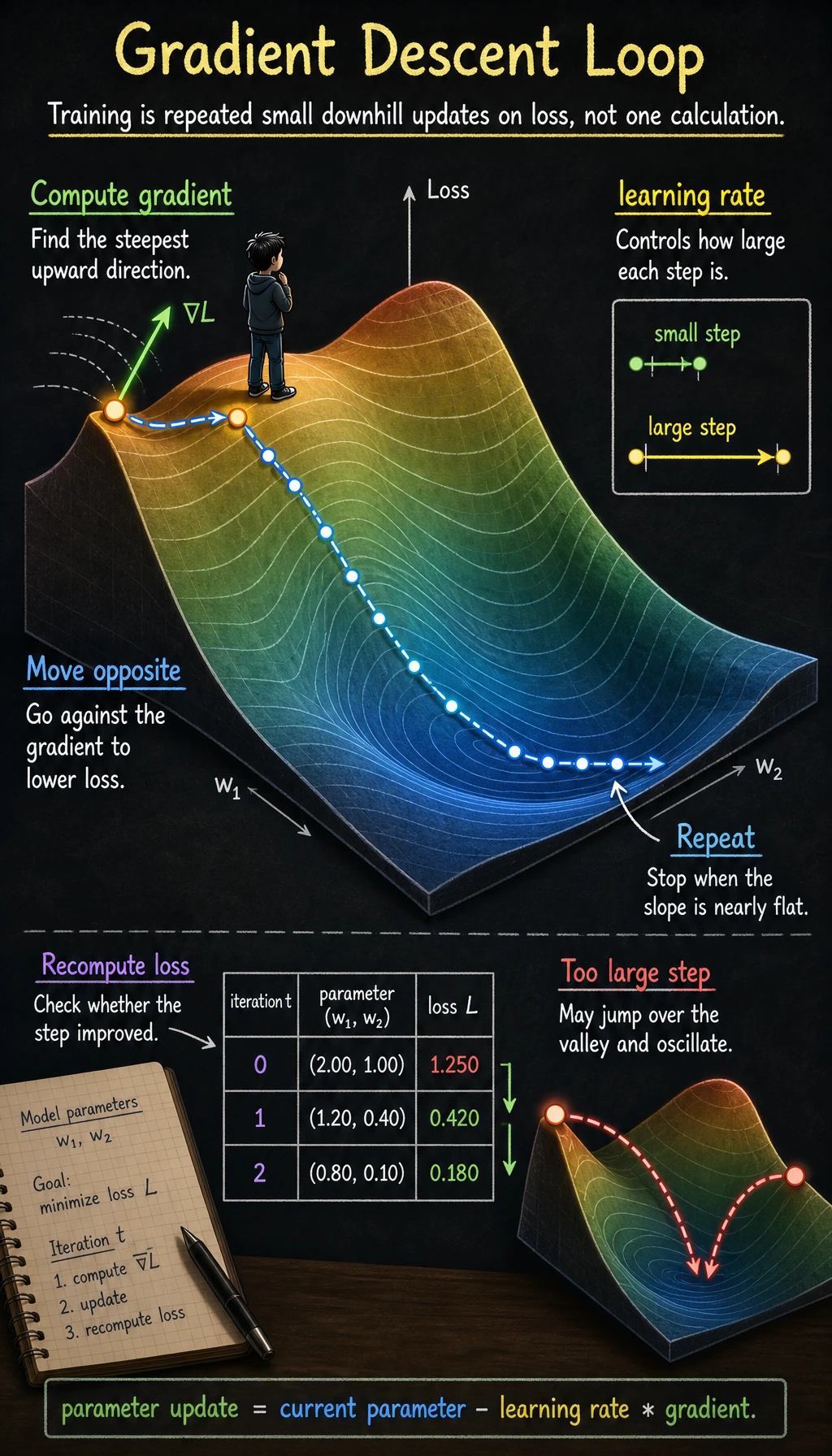
If you understand this section clearly, then later when you see optimizers, learning rates, and training processes, you won’t be left with just “memorizing the API.”

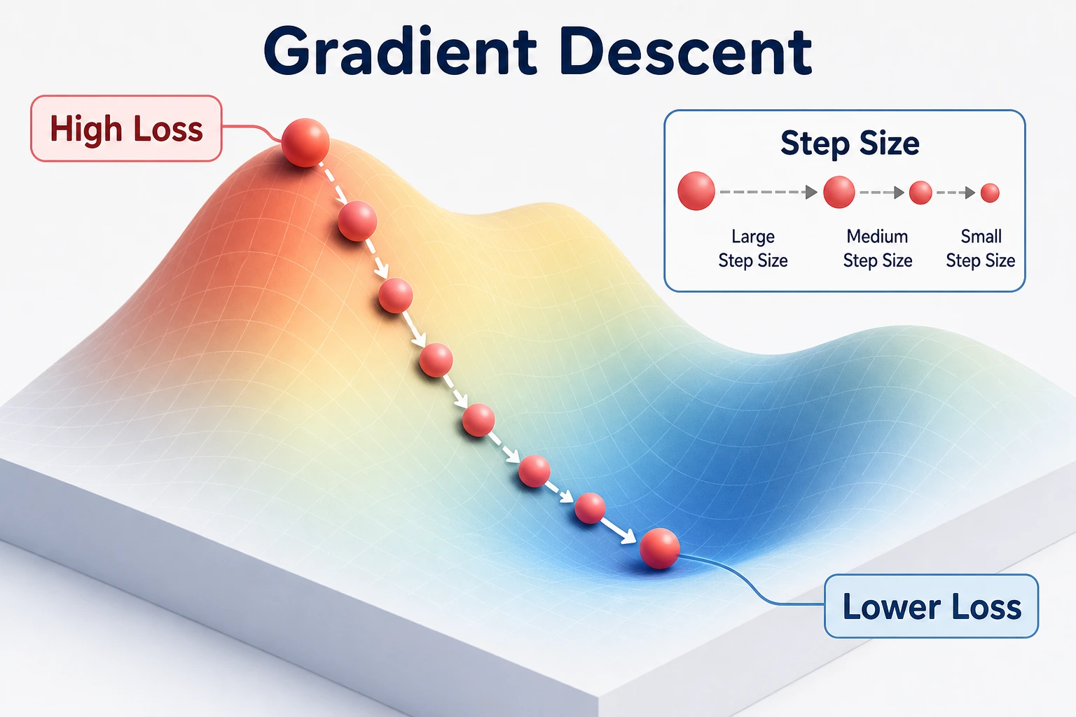
Intuition: Walking Down a Hill Blindfolded

Imagine you are standing on a mountain, blindfolded, and you want to reach the lowest point in the valley. What would you do?

1. Feel the ground with your feet: which direction is steepest? (= compute the gradient)
2. Take one step in the steepest downhill direction (= update parameters along the negative gradient direction)
3. Repeat until it feels flat all around (= the gradient is close to zero, meaning you have reached the minimum)

Why is this analogy especially important for beginners?

Because it helps you accept one thing first:

• Model training does not happen in one shot
• It improves little by little in a loss landscape where you cannot see the whole map

flowchart TD
    A["Initialize parameters<br/>（randomly standing on the mountain）"] --> B["Compute gradient<br/>（feel the slope of the ground）"]
    B --> C["Update parameters<br/>w = w - lr × gradient<br/>（take one step downhill）"]
    C --> D{"Has it converged?<br/>gradient ≈ 0?"}
    D -->|No| B
    D -->|Yes| E["Found the lowest point!"]

    style A fill:#e3f2fd,stroke:#1565c0,color:#333
    style E fill:#e8f5e9,stroke:#2e7d32,color:#333

---

Start by Understanding Through Code

The simplest example: finding the minimum of f(x) = x²

import numpy as np
import matplotlib.pyplot as plt

plt.rcParams['font.sans-serif'] = ['Arial Unicode MS']
plt.rcParams['axes.unicode_minus'] = False

# Target function
def f(x):
    return x ** 2

# Derivative
def df(x):
    return 2 * x

# Gradient descent
x = 4.0          # Initial position
lr = 0.3          # Learning rate
history = [x]     # Record the trajectory

for step in range(20):
    grad = df(x)              # Compute gradient
    x = x - lr * grad         # Update parameters
    history.append(x)
    if step < 8:
        print(f"Step {step+1}: x = {x:.4f}, f(x) = {f(x):.6f}, gradient = {grad:.4f}")

print(f"\nFinal: x = {x:.6f}, f(x) = {f(x):.10f}")

Visualize the descent process

x_plot = np.linspace(-5, 5, 200)

plt.figure(figsize=(10, 6))
plt.plot(x_plot, f(x_plot), 'steelblue', linewidth=2, label='f(x) = x²')

# Draw the position of each step
for i in range(len(history) - 1):
    plt.plot(history[i], f(history[i]), 'ro', markersize=8, alpha=0.5)
    plt.annotate('', xy=(history[i+1], f(history[i+1])),
                 xytext=(history[i], f(history[i])),
                 arrowprops=dict(arrowstyle='->', color='red', lw=1.5))

plt.plot(history[0], f(history[0]), 'ro', markersize=12, label=f'Start x={history[0]}')
plt.plot(history[-1], f(history[-1]), 'g*', markersize=15, label=f'End x={history[-1]:.2f}')

plt.xlabel('x')
plt.ylabel('f(x)')
plt.title('Gradient descent process: starting from x=4 and gradually reaching the minimum')
plt.legend()
plt.grid(True, alpha=0.3)
plt.show()

---

Learning Rate — The Most Important Hyperparameter

Learning rate too large vs too small

A more beginner-friendly analogy

The learning rate is very much like how big each step is when you walk downhill:

• Steps too small: you go down very slowly
• Steps too large: you may jump over the valley floor and oscillate back and forth

fig, axes = plt.subplots(1, 3, figsize=(18, 5))
x_plot = np.linspace(-5, 5, 200)

for ax, lr, title in zip(axes, [0.01, 0.3, 0.95],
                          ['Too small (lr=0.01)', 'Just right (lr=0.3)', 'Too large (lr=0.95)']):
    x = 4.0
    history = [x]
    for _ in range(30):
        x = x - lr * df(x)
        history.append(x)

    ax.plot(x_plot, f(x_plot), 'steelblue', linewidth=2)

    for i in range(min(len(history)-1, 20)):
        ax.plot(history[i], f(history[i]), 'ro', markersize=5, alpha=0.6)
        if i < len(history)-1:
            ax.plot([history[i], history[i+1]],
                    [f(history[i]), f(history[i+1])], 'r-', alpha=0.3)

    ax.set_title(f'{title}\nAfter 30 steps x={history[-1]:.4f}')
    ax.set_xlabel('x')
    ax.set_ylabel('f(x)')
    ax.set_ylim(-1, 30)
    ax.grid(True, alpha=0.3)

plt.suptitle('The effect of learning rate on gradient descent', fontsize=14)
plt.tight_layout()
plt.show()

Learning rate	Behavior	Problem
Too small (0.01)	Takes very tiny steps	Converges extremely slowly, may need tens of thousands of steps
Suitable (0.1~0.5)	Descends steadily	Ideal case
Too large (0.95+)	Oscillates back and forth	May never converge
Too large (>1.0)	Moves farther and farther away	Diverges (loss explodes)

When the learning rate exceeds 1.0

For f(x)=x², if lr > 1, the absolute value of x will keep getting larger with each step — the model “blows up” while learning.

x = 4.0
for i in range(5):
    x = x - 1.1 * (2*x)
    print(f"Step {i+1}: x={x:.2f}, f(x)={x**2:.2f}")
# x keeps getting larger!

---

Hands-on: Implement Gradient Descent from Scratch to Fit a Line

Problem setup

Use gradient descent to fit y = wx + b and find the best w and b.

# Generate data: y = 2x + 3 + noise
rng = np.random.default_rng(seed=42)
n = 100
X = rng.uniform(-5, 5, n)
y_true = 2 * X + 3 + rng.normal(size=n) * 1.5

plt.figure(figsize=(8, 5))
plt.scatter(X, y_true, alpha=0.5, s=30, color='steelblue')
plt.xlabel('x')
plt.ylabel('y')
plt.title('Data points (true relationship: y = 2x + 3 + noise)')
plt.grid(True, alpha=0.3)
plt.show()

Loss function

Mean Squared Error (MSE):

MSE = (1/n) × Σ (predicted value - true value)²

def predict(X, w, b):
    """Prediction function: y = wx + b"""
    return w * X + b

def mse_loss(X, y, w, b):
    """Mean squared error loss"""
    y_pred = predict(X, w, b)
    return np.mean((y_pred - y) ** 2)

def compute_gradients(X, y, w, b):
    """Compute gradients of the loss with respect to w and b"""
    y_pred = predict(X, w, b)
    n = len(y)
    dw = (2/n) * np.sum((y_pred - y) * X)
    db = (2/n) * np.sum(y_pred - y)
    return dw, db

Gradient descent training

# Initialize parameters
w = 0.0
b = 0.0
lr = 0.01
epochs = 200

# Record the training process
loss_history = []
w_history = []
b_history = []

for epoch in range(epochs):
    # 1. Compute loss
    loss = mse_loss(X, y_true, w, b)
    loss_history.append(loss)
    w_history.append(w)
    b_history.append(b)

    # 2. Compute gradients
    dw, db = compute_gradients(X, y_true, w, b)

    # 3. Update parameters
    w = w - lr * dw
    b = b - lr * db

    # Print progress
    if epoch % 40 == 0:
        print(f"Epoch {epoch:4d}: loss={loss:.4f}, w={w:.4f}, b={b:.4f}")

print(f"\nFinal result: w={w:.4f}, b={b:.4f}")
print(f"True parameters: w=2.0000, b=3.0000")

Visualize the training process

fig, axes = plt.subplots(1, 3, figsize=(18, 5))

# 1. Loss curve
axes[0].plot(loss_history, color='coral', linewidth=2)
axes[0].set_xlabel('Epoch')
axes[0].set_ylabel('MSE Loss')
axes[0].set_title('Training loss curve')
axes[0].grid(True, alpha=0.3)

# 2. Parameter convergence
axes[1].plot(w_history, label='w', color='steelblue', linewidth=2)
axes[1].plot(b_history, label='b', color='coral', linewidth=2)
axes[1].axhline(y=2.0, color='steelblue', linestyle='--', alpha=0.5, label='True w')
axes[1].axhline(y=3.0, color='coral', linestyle='--', alpha=0.5, label='True b')
axes[1].set_xlabel('Epoch')
axes[1].set_ylabel('Parameter value')
axes[1].set_title('Parameter convergence')
axes[1].legend()
axes[1].grid(True, alpha=0.3)

# 3. Fitting result
x_line = np.linspace(-5, 5, 100)
axes[2].scatter(X, y_true, alpha=0.4, s=20, color='gray')
axes[2].plot(x_line, 2*x_line + 3, 'g--', linewidth=2, label='True: y=2x+3')
axes[2].plot(x_line, w*x_line + b, 'r-', linewidth=2, label=f'Fit: y={w:.2f}x+{b:.2f}')
axes[2].set_xlabel('x')
axes[2].set_ylabel('y')
axes[2].set_title('Fitting result')
axes[2].legend()
axes[2].grid(True, alpha=0.3)

plt.tight_layout()
plt.show()

---

Three Variants of Gradient Descent

Batch Gradient Descent (BGD)

Use all data to compute the gradient at each step (the implementation above is BGD).

# BGD: use all n samples to compute the gradient
dw = (2/n) * np.sum((y_pred - y) * X)  # use all data

Stochastic Gradient Descent (SGD)

Use only one sample to compute the gradient at each step.

# SGD: use only 1 sample each time
rng = np.random.default_rng(seed=42)
i = rng.integers(0, n)
dw = 2 * (w * X[i] + b - y_true[i]) * X[i]

Mini-batch Gradient Descent (Mini-batch SGD)

Use a small batch of data at each step (for example, 32 samples) — the most commonly used.

# Mini-batch SGD
rng = np.random.default_rng(seed=42)
batch_size = 32
indices = rng.choice(n, batch_size, replace=False)
X_batch = X[indices]
y_batch = y_true[indices]
dw = (2/batch_size) * np.sum((w * X_batch + b - y_batch) * X_batch)

Comparison

Method	Each update uses	Best use
BGD	All data, exact gradient	Small datasets or teaching derivations
SGD	1 sample, noisy gradient	Understanding theory and stochastic behavior
Mini-batch	32-512 samples, stable enough	Most practical training loops

# Compare convergence curves of the three methods
fig, ax = plt.subplots(figsize=(10, 5))
rng = np.random.default_rng(seed=42)

for method, batch_size, color in [('BGD', n, 'steelblue'),
                                    ('Mini-batch(32)', 32, 'coral'),
                                    ('SGD', 1, 'gray')]:
    w, b = 0.0, 0.0
    lr = 0.01
    losses = []

    for epoch in range(200):
        if batch_size == n:
            idx = np.arange(n)
        else:
            idx = rng.choice(n, batch_size, replace=False)

        X_b, y_b = X[idx], y_true[idx]
        y_pred = w * X_b + b

        dw = (2/len(idx)) * np.sum((y_pred - y_b) * X_b)
        db = (2/len(idx)) * np.sum(y_pred - y_b)

        w -= lr * dw
        b -= lr * db

        losses.append(mse_loss(X, y_true, w, b))

    ax.plot(losses, label=method, color=color, linewidth=2,
            alpha=0.7 if method != 'SGD' else 0.4)

ax.set_xlabel('Epoch')
ax.set_ylabel('MSE Loss')
ax.set_title('Convergence comparison of the three gradient descent methods')
ax.legend()
ax.grid(True, alpha=0.3)
plt.show()

---

Local Minima and Saddle Points

Challenges of non-convex functions

# A function with multiple extrema
def tricky_f(x):
    return x**4 - 4*x**2 + 0.5*x

def tricky_df(x):
    return 4*x**3 - 8*x + 0.5

x_plot = np.linspace(-2.5, 2.5, 200)

plt.figure(figsize=(10, 5))
plt.plot(x_plot, tricky_f(x_plot), 'steelblue', linewidth=2)

# Start from different initial points
for x0, color in [(-2.0, 'red'), (0.5, 'green'), (2.0, 'orange')]:
    x = x0
    history = [x]
    for _ in range(100):
        x = x - 0.01 * tricky_df(x)
        history.append(x)

    for h in history[::5]:
        plt.plot(h, tricky_f(h), 'o', color=color, markersize=4, alpha=0.5)
    plt.plot(history[0], tricky_f(history[0]), 's', color=color, markersize=10,
             label=f'Start x={x0} → End x={history[-1]:.2f}')

plt.xlabel('x')
plt.ylabel('f(x)')
plt.title('Different starting points may find different extrema')
plt.legend()
plt.grid(True, alpha=0.3)
plt.show()

Interpretation: Different starting points may “walk downhill” to different valleys (local minima). In deep learning, the good news is that local minima in high-dimensional spaces are usually good enough.

Saddle points

flowchart LR
    A["Local minimum<br/>Higher all around<br/>Getting stuck there is not too bad"]
    B["Saddle point<br/>Rises in some directions and falls in others<br/>Gradient is zero but it is not the lowest point"]

    style A fill:#fff3e0,stroke:#e65100,color:#333
    style B fill:#ffebee,stroke:#c62828,color:#333

In high-dimensional spaces, saddle points are more common than local minima. Modern optimizers such as Adam can help jump over saddle points through momentum mechanisms.

---

After learning this, what questions should you bring to the next section?

After looking at gradient descent, the most valuable questions to bring to the next section are:

1. If a network has many layers, how does the gradient flow back layer by layer?
2. Why can loss.backward() compute the gradients of all parameters at once?
3. How exactly does the chain rule work in a complex network?

These questions will naturally lead you to:

• 4.3.5 Preview of the chain rule and backpropagation

Connecting to what comes next

• Next section: Chain rule — how to efficiently compute the gradient of each parameter in a complex network
• Stop 5: Training linear regression and logistic regression both use gradient descent
• Stop 6: optimizer.step() in PyTorch performs one gradient descent step
• Advanced optimizers: Adam and AdamW are improved versions of gradient descent (adaptive learning rate + momentum)

---

Evidence to Keep

Keep this page’s proof of learning as a small evidence card:

Function

objective, loss, derivative, gradient, or chain-rule expression

Calculation

numeric derivative, gradient step, or backprop trace

Output

slope, gradient vector, updated parameter, or loss change

Failure Check

sign error, learning rate too large, local slope misunderstanding, or broken chain

Expected Output

calculation trace showing how a parameter changes

Summary

Concept	Intuition
Gradient descent	Move step by step along the negative gradient direction toward the minimum
Learning rate	How far you move each step (too large causes oscillation, too small is too slow)
BGD	Compute gradients using all data (accurate but slow)
Mini-batch SGD	Use a small batch of data (most commonly used)
Local minimum	A point that is not globally optimal but has zero gradient

What you should take away from this section

• The most important intuition of gradient descent is “update step by step in the direction that decreases the loss”
• The learning rate determines “how far each step moves”
• Training a model is, in essence, a repeated process of “look at the gradient -> take a step -> look again”

Hands-on Exercises

Exercise 1: Tune the learning rate

Modify the code in Section 4.3, train with lr=0.001, 0.01, 0.1, and 0.5 respectively, and plot four loss curves for comparison.

Exercise 2: Fit a quadratic function from scratch

Use gradient descent to fit y = ax² + bx + c and find the best a, b, and c. Data:

X = np.linspace(-3, 3, 100)
rng = np.random.default_rng(seed=42)
y = 0.5 * X**2 - 2 * X + 1 + rng.normal(size=100) * 0.5

Exercise 3: Visualize 2D gradient descent

For f(x, y) = x² + 2y², start from (4, 3) and run gradient descent, then draw the descent path on a contour plot.

Reference implementation and walkthrough

• With learning rates 0.001, 0.01, 0.1, and 0.5, expect very slow improvement at 0.001, steadier improvement around 0.01 or 0.1, and possible oscillation or divergence at 0.5 depending on scaling.
• For the quadratic fit, the learned parameters should move close to the data-generating values a≈0.5, b≈-2, and c≈1, with noise preventing perfect equality.
• For f(x,y)=x^2+2y^2, the update moves faster along the y direction because its gradient component is 4y. The path should curve toward the origin.