5.1.6 Scikit-learn and Matplotlib Hands-on Workshop

Section focus

This is a follow-along workshop. The goal is not to add more theory, but to help you run a complete classic machine learning workflow by yourself: load data, visualize first, split data, train a model, evaluate it, improve it safely, and save it.

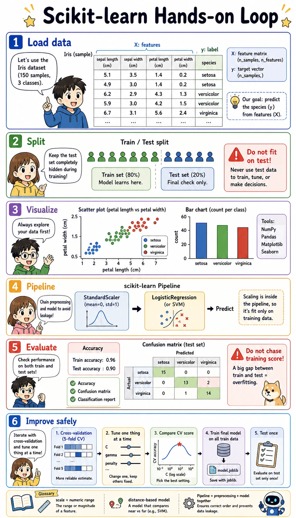
Learning objectives

• Understand what X, y, X_train, X_test, y_train, and y_test mean in real code
• Use Matplotlib to read data and model results before trusting a score
• Build a sklearn Pipeline that combines preprocessing and a model
• Compare training and test scores without being fooled by overfitting
• Use cross-validation to tune one thing at a time
• Save and reload a trained Pipeline with joblib

Prepare one runnable cell

Create a new notebook or Python file, then run this setup first.

import numpy as np
import matplotlib.pyplot as plt

from sklearn.datasets import load_wine
from sklearn.model_selection import train_test_split, cross_val_score
from sklearn.pipeline import make_pipeline
from sklearn.preprocessing import StandardScaler
from sklearn.linear_model import LogisticRegression
from sklearn.metrics import ConfusionMatrixDisplay, classification_report

np.set_printoptions(precision=3, suppress=True)

If import sklearn fails, install the packages in the same Python environment:

python -m pip install --upgrade scikit-learn matplotlib joblib

pip installs packages. python -m pip means “use the pip that belongs to this exact Python interpreter,” which avoids the common mistake of installing into one environment and running code in another.

---

Load data: separate features and labels

In sklearn examples, you will see X and y all the time:

• X is the feature matrix. Each row is one sample, and each column is one input feature.
• y is the target vector. Each value is the answer label we want the model to learn.
• X.shape tells you (number_of_samples, number_of_features).
• y.shape tells you how many labels you have.

wine = load_wine()
X = wine.data
y = wine.target

print("X shape:", X.shape)
print("y shape:", y.shape)
print("Feature names:", wine.feature_names[:5], "...")
print("Class names:", wine.target_names.tolist())
print("First sample features:", np.round(X[0], 2))
print("First sample label:", y[0], "=>", wine.target_names[y[0]])

Expected output:

X shape: (178, 13)
y shape: (178,)
Feature names: ['alcohol', 'malic_acid', 'ash', 'alcalinity_of_ash', 'magnesium'] ...
Class names: ['class_0', 'class_1', 'class_2']
First sample features: [ 14.23   1.71   2.43  15.6  127.     2.8    3.06   0.28   2.29   5.64   1.04   3.92 1065.  ]
First sample label: 0 => class_0

Beginner checkpoint

Before training any model, always answer three questions: “What is one row? What is one column? What is the label?” If those are unclear, the score will not mean much yet.

---

Matplotlib basics: read the chart before the model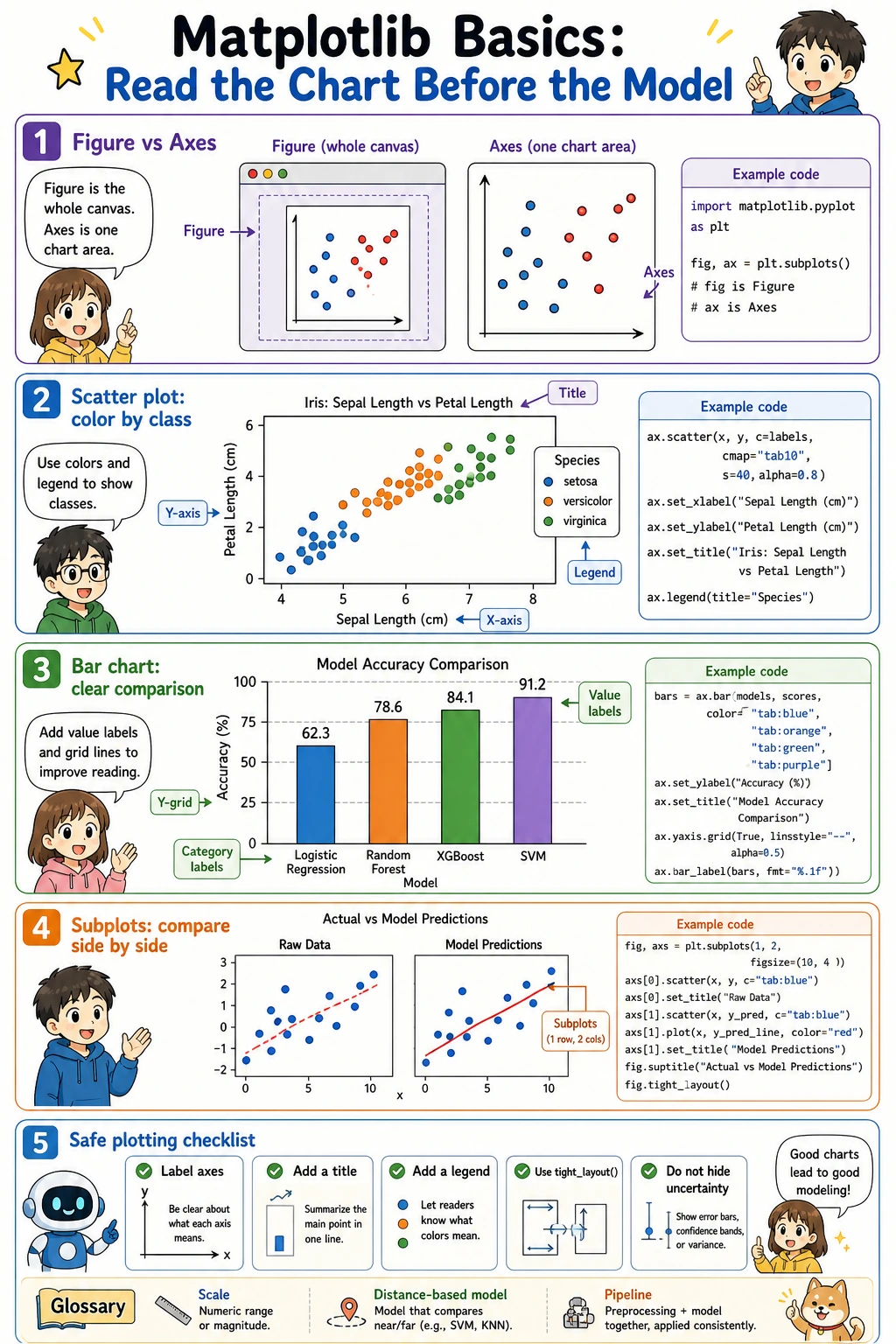

Matplotlib has two words that confuse beginners:

• Figure: the whole canvas.
• Axes: one chart area inside the canvas.

Most beginner code can follow this pattern:

fig, ax = plt.subplots(figsize=(6, 4))
ax.scatter(x_values, y_values)
ax.set_xlabel("x-axis label")
ax.set_ylabel("y-axis label")
ax.set_title("Chart title")
ax.grid(True, alpha=0.3)
plt.tight_layout()
plt.show()

Now draw two Wine features:

feature_x = 0  # alcohol
feature_y = 6  # flavanoids

fig, ax = plt.subplots(figsize=(7, 5))
scatter = ax.scatter(
    X[:, feature_x],
    X[:, feature_y],
    c=y,
    cmap="viridis",
    s=45,
    alpha=0.85,
)

ax.set_xlabel(wine.feature_names[feature_x])
ax.set_ylabel(wine.feature_names[feature_y])
ax.set_title("Wine data: two-feature view")
ax.grid(True, alpha=0.3)
ax.legend(
    handles=scatter.legend_elements()[0],
    labels=wine.target_names.tolist(),
    title="Class",
)

plt.tight_layout()
plt.show()

What to observe:

• Are the classes already somewhat separated?
• Are there overlapping regions?
• Does one feature have a much larger numeric range than another feature?

This is why visualization matters: it gives you a first feeling for whether the model is solving an easy or difficult problem.

---

Split data: keep the test set hidden

train_test_split creates a training set and a test set.

• Training set: the model is allowed to learn from it.
• Test set: the model should only see it at the final evaluation step.
• stratify=y: keep class proportions similar in train and test.
• random_state: make the split reproducible.

X_train, X_test, y_train, y_test = train_test_split(
    X,
    y,
    test_size=0.2,
    random_state=42,
    stratify=y,
)

print("X_train:", X_train.shape, "y_train:", y_train.shape)
print("X_test: ", X_test.shape, "y_test: ", y_test.shape)

Expected output:

X_train: (142, 13) y_train: (142,)
X_test:  (36, 13) y_test:  (36,)

The most common beginner mistake

Do not run fit on the test set. The test set is your final exam. If preprocessing or tuning learns from the test set, the reported score becomes too optimistic.

---

Build a Pipeline: preprocessing plus model

Many models, such as logistic regression, SVM, and KNN, are sensitive to feature scale. The Wine dataset has columns with very different units, so we put StandardScaler before the model.

model = make_pipeline(
    StandardScaler(),
    LogisticRegression(max_iter=1000, random_state=42),
)

model.fit(X_train, y_train)

train_score = model.score(X_train, y_train)
test_score = model.score(X_test, y_test)

print(f"Train accuracy: {train_score:.1%}")
print(f"Test accuracy:  {test_score:.1%}")

Expected output:

Train accuracy: 100.0%
Test accuracy:  100.0%

Pipeline matters because it keeps the correct order:

1. On training data: StandardScaler.fit_transform then model fit
2. On test data: StandardScaler.transform then model predict

That tiny difference prevents data leakage.

---

Predict and inspect concrete examples

A score is useful, but beginners should also look at a few actual predictions.

y_pred = model.predict(X_test)
proba = model.predict_proba(X_test[:5])

for i in range(5):
    predicted_name = wine.target_names[y_pred[i]]
    true_name = wine.target_names[y_test[i]]
    confidence = proba[i].max()
    print(f"Sample {i}: predicted={predicted_name}, true={true_name}, confidence={confidence:.1%}")

Example output:

Sample 0: predicted=class_0, true=class_0, confidence=99.9%
Sample 1: predicted=class_1, true=class_1, confidence=99.9%
Sample 2: predicted=class_0, true=class_0, confidence=99.5%
Sample 3: predicted=class_1, true=class_1, confidence=99.7%
Sample 4: predicted=class_2, true=class_2, confidence=99.9%

predict returns the final class. predict_proba returns the probability distribution over classes. Probability is useful when a business process needs thresholds, manual review, or risk ranking.

---

Evaluate with a confusion matrix and report

Accuracy alone hides which classes are confused with each other. A confusion matrix shows actual labels on one axis and predicted labels on the other axis.

fig, ax = plt.subplots(figsize=(5, 5))
ConfusionMatrixDisplay.from_estimator(
    model,
    X_test,
    y_test,
    display_labels=wine.target_names,
    cmap="Blues",
    ax=ax,
    colorbar=False,
)
ax.set_title("Confusion matrix on test set")
plt.tight_layout()
plt.show()

print(classification_report(y_test, y_pred, target_names=wine.target_names))

What to read:

• Diagonal cells are correct predictions.
• Off-diagonal cells are mistakes.
• Precision asks: “Among predicted class A, how many were really A?”
• Recall asks: “Among real class A, how many did we catch?”
• F1 combines precision and recall.

---

Compare several models with the same workflow

Because sklearn has a unified API, model comparison is very practical.

from sklearn.tree import DecisionTreeClassifier
from sklearn.neighbors import KNeighborsClassifier
from sklearn.svm import SVC

models = {
    "Logistic Regression": make_pipeline(
        StandardScaler(),
        LogisticRegression(max_iter=1000, random_state=42),
    ),
    "Decision Tree": DecisionTreeClassifier(max_depth=4, random_state=42),
    "KNN": make_pipeline(StandardScaler(), KNeighborsClassifier(n_neighbors=5)),
    "SVM": make_pipeline(StandardScaler(), SVC(kernel="rbf", C=1.0, gamma="scale")),
}

results = {}
for name, clf in models.items():
    clf.fit(X_train, y_train)
    results[name] = {
        "train": clf.score(X_train, y_train),
        "test": clf.score(X_test, y_test),
    }
    print(f"{name:20s} train={results[name]['train']:.1%} test={results[name]['test']:.1%}")

Example output:

Logistic Regression  train=100.0% test=100.0%
Decision Tree        train=99.3% test=94.4%
KNN                  train=97.9% test=97.2%
SVM                  train=100.0% test=100.0%

Now draw the comparison:

fig, ax = plt.subplots(figsize=(9, 5))
names = list(results.keys())
x = np.arange(len(names))
width = 0.35

train_scores = [results[name]["train"] for name in names]
test_scores = [results[name]["test"] for name in names]

bars_train = ax.bar(x - width / 2, train_scores, width, label="Train", color="steelblue")
bars_test = ax.bar(x + width / 2, test_scores, width, label="Test", color="coral")

ax.set_xticks(x)
ax.set_xticklabels(names, rotation=15, ha="right")
ax.set_ylabel("Accuracy")
ax.set_title("Model comparison on Wine dataset")
ax.set_ylim(0.8, 1.05)
ax.legend()
ax.grid(axis="y", alpha=0.3)
ax.bar_label(bars_train, fmt="%.2f", padding=3)
ax.bar_label(bars_test, fmt="%.2f", padding=3)

plt.tight_layout()
plt.show()

If train score is much higher than test score, suspect overfitting. If both scores are low, suspect underfitting, weak features, or an unsuitable model.

---

Tune safely with cross-validation

Do not tune hyperparameters directly on the test set. Use cross-validation on the training set.

candidates = [0.01, 0.1, 1.0, 10.0, 100.0]

for C in candidates:
    clf = make_pipeline(
        StandardScaler(),
        LogisticRegression(C=C, max_iter=1000, random_state=42),
    )
    scores = cross_val_score(clf, X_train, y_train, cv=5, scoring="accuracy")
    print(f"C={C:<6} CV accuracy={scores.mean():.1%} ± {scores.std():.1%}")

Example output:

C=0.01   CV accuracy=95.8% ± 3.1%
C=0.1    CV accuracy=98.6% ± 1.8%
C=1.0    CV accuracy=98.6% ± 1.8%
C=10.0   CV accuracy=97.9% ± 2.6%
C=100.0  CV accuracy=97.9% ± 2.6%

The habit is more important than this exact result:

1. Split off a test set and do not touch it.
2. Tune with cross-validation on the training set.
3. Choose the best setting.
4. Train one final model on all training data.
5. Evaluate on the test set once.

---

Save and reload the final Pipeline

import joblib

final_model = make_pipeline(
    StandardScaler(),
    LogisticRegression(C=1.0, max_iter=1000, random_state=42),
)
final_model.fit(X_train, y_train)

joblib.dump(final_model, "wine_classifier.joblib")
loaded_model = joblib.load("wine_classifier.joblib")

same_predictions = np.array_equal(
    final_model.predict(X_test),
    loaded_model.predict(X_test),
)

print("Loaded model test accuracy:", f"{loaded_model.score(X_test, y_test):.1%}")
print("Predictions are identical:", same_predictions)

Expected output:

Loaded model test accuracy: 100.0%
Predictions are identical: True

Security note

Only load joblib or pickle files you trust. Loading serialized Python objects can execute code.

---

Evidence to Keep

Keep this page’s proof of learning as a small evidence card:

Ml Problem

supervised, unsupervised, evaluation, or feature-engineering task

Baseline

simplest sklearn/modeling loop and fixed train/test split

Output

prediction, metric, chart, or model decision note

Failure Check

data leakage, unclear target, weak baseline, or metric mismatch

Expected Output

minimal ML loop with metric and one failure observation

Common errors and quick fixes

Error / symptom	Likely cause	Fix
NameError: name 'X_train' is not defined	You skipped the split cell	Run the data loading and train_test_split cells first
ValueError: Found input variables with inconsistent numbers of samples	X and y lengths do not match	Print X.shape and y.shape before splitting
Very high train score, much lower test score	Overfitting	Reduce model complexity, use cross-validation, add data, or improve features
Good notebook score, bad real usage	Data leakage or mismatched preprocessing	Save and use the whole Pipeline, not only the model
Chart labels overlap	Figure too small or layout not adjusted	Increase figsize, rotate labels, use plt.tight_layout()

Hands-on task

Repeat the whole workflow with load_iris():

1. Print X.shape, y.shape, feature names, and class names.
2. Draw a scatter plot using two features.
3. Split with train_test_split(..., stratify=y).
4. Train a Pipeline(StandardScaler(), LogisticRegression(...)).
5. Print train/test accuracy.
6. Draw a confusion matrix.
7. Tune C with cross-validation.
8. Save and reload the model with joblib.

Operation guide and checkpoints

1. load_iris() should give 150 rows, 4 numeric features, and 3 class names. If X.shape[0] and y.shape[0] differ, the feature/label split is wrong.
2. The scatter plot should show that some feature pairs separate the classes better than others. Treat the plot as a structure check, not as proof that the model is good.
3. stratify=y keeps the class ratios stable in train and test, which matters even for a small balanced dataset.
4. The Pipeline should include both StandardScaler() and LogisticRegression(...) so scaling is fitted only from the training data.
5. Train and test accuracy should be close. If train is much higher than test, inspect overfitting or an unstable split.
6. The confusion matrix tells you which class pairs are confused. Use it before changing the model blindly.
7. Tune C with cross-validation on the training side, then check the test set once. Do not pick C by repeatedly looking at the test score.
8. After joblib reload, predictions should match the original model. Only load serialized files you trust.

What should you take away from this workshop?

If Chapter 5 has one hands-on loop, it is this:

Look at the data first, split before fitting, use Pipeline for preprocessing plus model, evaluate on hidden data, improve with cross-validation, and save the complete workflow.