
4.2.6 Historical Main Line of Probability and Statistics: Bayes, MLE, EM, and Information Theory
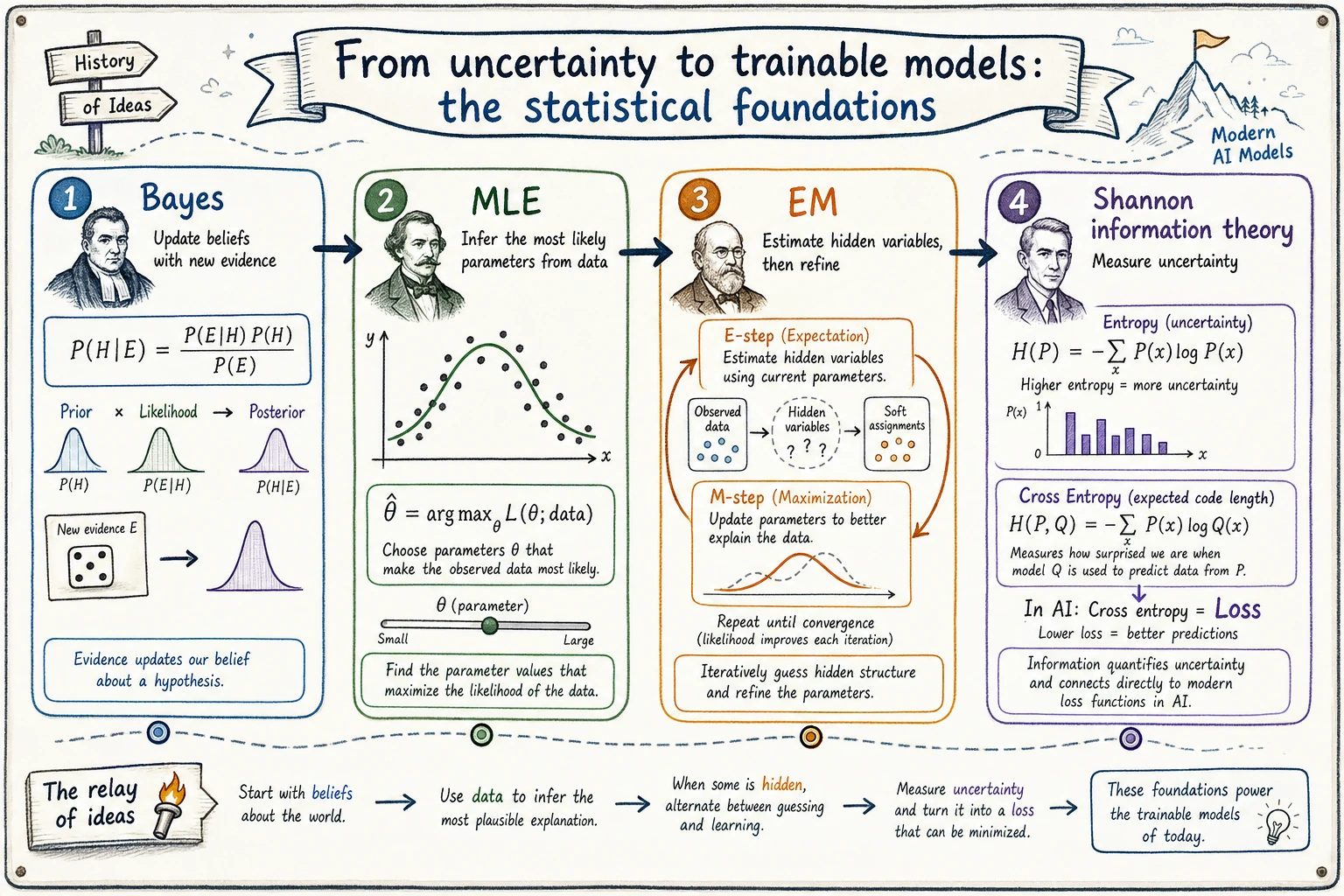
Why do these old ideas still keep showing up in AI today?
Section titled “Why do these old ideas still keep showing up in AI today?”AI models may look modern, but underneath they have always been dealing with three classic problems:
| Old problem | Corresponding idea | Where it appears today |
|---|---|---|
| New evidence arrives—should the judgment change? | Bayes’ rule | Classification probabilities, diagnostic systems, recommender systems, RAG confidence |
| Nobody tells me the parameters—how can I infer them from data? | Maximum likelihood estimation, MLE | Loss functions, logistic regression, language model training |
| Some variables are invisible—can we still estimate the parameters? | EM algorithm | Clustering, topic models, latent variable models |
| How uncertain is the prediction, really? | Information theory | Entropy, cross entropy, KL divergence, classification loss |
So these milestones are not “old relics from math class.” They are still the underlying language of many modern algorithms.
Bayes: when new evidence arrives, the judgment updates
Section titled “Bayes: when new evidence arrives, the judgment updates”Bayes’ rule is easiest to understand as “a detective updating a judgment.”
At the beginning, you have an initial judgment, called the prior. Later, when new evidence appears, you update that judgment into the posterior.
prior judgment + new evidence -> updated judgmentIn AI projects, this intuition shows up all the time:
- Spam detection: after seeing keywords, does the probability that an email is spam change?
- Medical decision support: after seeing a new test result, does the likelihood of a disease change?
- RAG question answering: is the retrieved evidence strong enough, or should the system answer “uncertain”?
The most important thing about Bayes’ rule is not what the formula looks like, but this habit:
Do not treat your first impression as final. Evidence can change probabilities.
MLE: infer the most likely parameters from data
Section titled “MLE: infer the most likely parameters from data”Maximum likelihood estimation answers a different question:
If the data has already happened, which set of parameters is most likely to have generated it?
You can think of MLE as “working backward from the clues”:
| Detective story | Statistical inference |
|---|---|
| Traces are left at the scene | We observe data |
| We do not know what really happened | We do not know the true parameters |
| Find the story that best explains the traces | Find the parameters that best explain the data |
A minimal example is flipping a coin. You flip it 10 times and get heads 8 times.
What is the most likely value of the heads probability p?
Intuitively, it is p = 0.8.
MLE turns this into mathematics:
import numpy as np
heads = 8tails = 2p_values = np.linspace(0.01, 0.99, 99)
likelihood = p_values**heads * (1 - p_values)**tailsp_mle = p_values[np.argmax(likelihood)]
print(round(p_mle, 2))
This idea will appear again and again in Chapter 5 logistic regression, Chapter 6 cross entropy, and Chapter 7 language model training.
EM: even invisible variables can be guessed first and then refined
Section titled “EM: even invisible variables can be guessed first and then refined”The EM algorithm solves a more difficult case:
If some causes that affect the data are hidden, can we still estimate the parameters?
For example, you may see a batch of user behavior data but not know which user group each user belongs to; or you may see a collection of texts but not know the latent topic of each article.
The intuition of EM is like a two-step loop:
| Step | What it does | Analogy |
|---|---|---|
| E-step | First, using the current parameters, guess what the hidden variables might be | First guess which suspect a clue belongs to |
| M-step | Then, based on the guessed hidden variables, update the parameters | Recompute each suspect’s features based on the new grouping |
It tells beginners something very important:
Not all training problems can be solved in one step. Many models reach a solution by iterating toward it with incomplete information.
Shannon: uncertainty can also be computed
Section titled “Shannon: uncertainty can also be computed”In 1948, Shannon’s information theory turned “information content” and “entropy” into quantities we can calculate. This is crucial for AI, because model training often asks:
- How messy is the prediction distribution?
- How far is the model’s prediction from the true label?
- Which token is more surprising?
For example, cross entropy in a classification task can be understood as:
How much information cost the model pays when it uses its own probability distribution to explain the true answer.
That is why you keep seeing this in deep learning:
loss = cross_entropy(prediction, label)It looks like a loss function on the surface, but underneath it is connected to information theory.
Assigning historical milestones to course chapters
Section titled “Assigning historical milestones to course chapters”| Historical milestone | First idea | Course link |
|---|---|---|
| Bayes’ rule | New evidence updates the judgment | 2.2 Probability foundations, 5.1 Machine learning basics |
| Maximum likelihood estimation | Find the parameters that best explain the data | 2.4 Statistical inference, 5.2 Supervised learning |
| EM algorithm | When there are hidden variables, guess first and then refine | 2.4 Statistical inference, 5.3 Unsupervised learning |
| Shannon information theory | Uncertainty can be measured | 2.5 Information theory, 6.2 PyTorch loss |
| MCMC / Bayesian inference | Complex posteriors can be approximated by sampling | Elective extension, background in probabilistic inference |
| Pearl causality | Correlation is not the same as causation | Chapter 3 data analysis, Chapter 9 decision systems background |
The intuition you should have after learning this section
Section titled “The intuition you should have after learning this section”These historical lines are really helping you build the “language of judgment” in AI:
- Bayes tells you that judgments change with evidence
- MLE tells you that training can be seen as inferring parameters from data
- EM tells you that hidden information can be approximated iteratively
- Shannon tells you that uncertainty, error, and information gaps can be quantified
When you later see probability, likelihood, entropy, cross entropy, or KL divergence, do not think of them only as formulas.
They are all answering the same question underneath:
In an uncertain world, how does a model make judgments that are computable, updatable, and optimizable?
Evidence to Keep
Section titled “Evidence to Keep”Keep this page’s proof of learning as a small evidence card:
- Random Process
- event, distribution, sample, likelihood, entropy, or Bayes update
- Simulation Or Formula
- code or formula used to make uncertainty visible
- Output
- probability, sample statistic, interval, entropy, or updated belief
- Failure Check
- base-rate confusion, p-value misuse, sample bias, or mixing probability with certainty
- Expected Output
- numeric result plus interpretation in plain language
Review notes and pass criteria
- A passing review should translate every number back into a judgment: what changed, what stayed uncertain, and what evidence would update the conclusion.
- Check one Bayes update, one likelihood choice, and one entropy or cross-entropy value. If the result is only a formula with no plain-language interpretation, the work is not finished.
- Keep one failure example where probability is treated as certainty or where a base rate is ignored. This is the most common practical mistake.
- The page is complete when you can explain why probability is the shared language behind data analysis, ML training, loss functions, and model evaluation.