4.1.2 Vectors: The Basic Unit of the AI World

Learning approach

You do not need to “prove theorems” in this chapter. You only need to understand the intuition and know how to implement it in code. Each concept comes with visualization and NumPy code. It is okay if you do not fully understand the formulas—just understand the diagrams and code.

Learning Objectives

• Intuitively understand what a vector is (direction + magnitude)
• Master vector addition and scalar multiplication
• Understand the meaning of dot product
• Master cosine similarity — the most commonly used similarity measure in AI
• Implement all vector operations with NumPy

First, set a very important learning expectation

Although this section includes code, the code is not there to replace understanding. It is more like doing two things:

• Helping you turn abstract objects into something visible
• Helping you check whether your intuition is correct

If you finish this section and still cannot solve problems fluently right away, that is completely normal. A more important standard is:

• Can you write a “real-world object” as a vector?
• Can you clearly explain what dot product and cosine similarity are comparing?
• Can you connect them to AI scenarios such as recommendation, retrieval, and RAG?

---

First, build a map

The most important thing in this section is not memorizing terms, but first grasping the main thread:

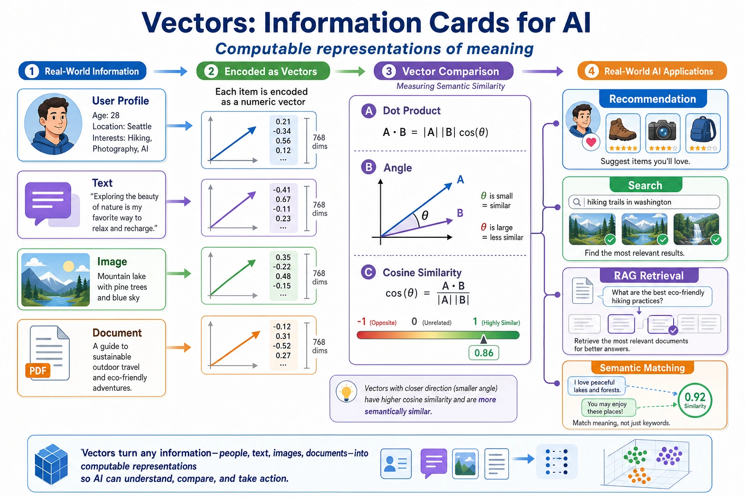
You can understand this lesson as:

• The first half answers “how to write an object as a vector”
• The second half answers “how to compare whether two vectors are similar”

Terms to Keep Handy

Term	What it means	Why beginners often need it
scalar	A single number, such as 2 or 0.5	Scalar multiplication means “use one number to scale the whole vector.”
dimension	The number of components in a vector	[90, 85, 92] has 3 dimensions because it has 3 numbers.
shape	NumPy’s description of array structure	(3,), (1, 3), and (3, 1) all hold 3 numbers but behave differently in multiplication.
norm	Vector length	np.linalg.norm(a) tells you how long or strong a vector is.
NLP	Natural Language Processing	Text vectors and word vectors are important examples of vectors in AI.
vector database	A database optimized for storing and searching vectors	It powers retrieval in many RAG and semantic search systems.

Read this table as a safety net, not as vocabulary to memorize. When a later code example uses one of these words, return here and reconnect it to the current operation.

What Is a Vector?

Intuitive Understanding

A vector = an ordered set of numbers.

A more beginner-friendly analogy

If this is your first time learning vectors, and “direction + magnitude” still feels a bit abstract, you can think of it as:

• An information card for an object

For example, a model evaluation run:

• Accuracy 0.86
• Latency 120 ms
• Memory 3.8 GB

Arrange these items in a fixed order, and you get an information card that a computer can process:

• [0.86, 120, 3.8]

So the most basic meaning of a vector is not a “geometric shape,” but:

A stable way to write an object as a sequence of numbers.

That is all. In AI, vectors are everywhere:

AI scenario	Vector representation	Dimension
One model run	[accuracy, latency_ms, memory_gb] = [0.86, 120, 3.8]	3D
The color of a pixel	[R, G, B] = [255, 128, 0]	3D
The meaning of a word (word vector)	[0.2, -0.5, 0.8, …]	Usually 100–300D
An image (flattened)	[pixel1, pixel2, …, pixeln]	Tens of thousands to millions of dimensions

  root((Vectors in AI))
    Data representation
      Each row of data is a vector
      Images are pixel vectors
      Text is word vectors
    Similarity computation
      Recommendation systems
      Search engines
      Face recognition
    Model parameters
      Neural network weights
      Gradients are also vectors

Geometric Intuition

In 2D space, a vector can be drawn as a line segment with an arrow — it has both direction and magnitude (length).

import numpy as np
import matplotlib.pyplot as plt

plt.rcParams['font.sans-serif'] = ['Arial Unicode MS']
plt.rcParams['axes.unicode_minus'] = False

# Define two 2D vectors
a = np.array([3, 2])
b = np.array([1, 4])

# Plot vectors
fig, ax = plt.subplots(figsize=(6, 6))
ax.quiver(0, 0, a[0], a[1], angles='xy', scale_units='xy', scale=1,
          color='steelblue', linewidth=2, label=f'a = {a}')
ax.quiver(0, 0, b[0], b[1], angles='xy', scale_units='xy', scale=1,
          color='coral', linewidth=2, label=f'b = {b}')

ax.set_xlim(-1, 6)
ax.set_ylim(-1, 6)
ax.set_aspect('equal')
ax.grid(True, alpha=0.3)
ax.axhline(y=0, color='k', linewidth=0.5)
ax.axvline(x=0, color='k', linewidth=0.5)
ax.legend(fontsize=12)
ax.set_title('Geometric representation of 2D vectors')
plt.show()

Interpretation: vector a = [3, 2] starts at the origin, moves 3 steps to the right and 2 steps up.

How should you understand high-dimensional vectors?

Vectors in AI are often hundreds or thousands of dimensions, so they cannot be drawn. But the mathematical operations are exactly the same — a vector is just a sequence of numbers, and all the rules apply to any dimension.

From a Real Data Record to a Vector

A point where beginners often get stuck is this: they know “a vector is a sequence of numbers,” but they do not know how that connects to real data.

import numpy as np

model_run = {
    "accuracy": 0.86,
    "latency_ms": 120,
    "memory_gb": 3.8,
}

model_vector = np.array([
    model_run["accuracy"],
    model_run["latency_ms"],
    model_run["memory_gb"],
])

print("Model run vector:", model_vector)
print("Vector shape:", model_vector.shape)  # (3,)

The essence here is:

• In the real world, there are “meaningful fields”
• In the computer, they must become a “fixed-order numeric array”

Once you write an object as a vector, you can start doing mathematical operations.

weights = np.array([0.7, -0.002, -0.03])
score = model_vector @ weights
print("Deployment score:", round(score, 3))  # 0.248

This already connects to a main thread in machine learning:

• Data is a vector
• Rules are also vectors
• If you take the dot product of the two, you get a score

---

Basic Vector Operations

Vector Addition

Adding two vectors = adding the numbers at corresponding positions.

a = np.array([3, 2])
b = np.array([1, 4])

# Vector addition
c = a + b
print(f"a + b = {c}")  # [4, 6]

Geometric meaning: place b at the end of a, and the result points to the final endpoint.

fig, ax = plt.subplots(figsize=(7, 7))

# Plot a
ax.quiver(0, 0, a[0], a[1], angles='xy', scale_units='xy', scale=1,
          color='steelblue', linewidth=2, label=f'a = {a}')
# Plot b (starting from the end of a)
ax.quiver(a[0], a[1], b[0], b[1], angles='xy', scale_units='xy', scale=1,
          color='coral', linewidth=2, label=f'b = {b}')
# Plot a + b
ax.quiver(0, 0, c[0], c[1], angles='xy', scale_units='xy', scale=1,
          color='green', linewidth=2.5, label=f'a + b = {c}')

ax.set_xlim(-1, 7)
ax.set_ylim(-1, 8)
ax.set_aspect('equal')
ax.grid(True, alpha=0.3)
ax.legend(fontsize=11)
ax.set_title('Vector addition: head-to-tail')
plt.show()

Scalar Multiplication

Multiplying a vector by a number = multiplying each component by that number.

a = np.array([3, 2])

# Scalar multiplication
print(f"2 * a = {2 * a}")     # [6, 4]  —— same direction, twice the length
print(f"0.5 * a = {0.5 * a}") # [1.5, 1.0]  —— same direction, half the length
print(f"-1 * a = {-1 * a}")   # [-3, -2]  —— reversed direction

fig, ax = plt.subplots(figsize=(8, 6))

vectors = [
    (a, 'steelblue', f'a = {a}'),
    (2 * a, 'green', f'2a = {2*a}'),
    (0.5 * a, 'orange', f'0.5a = {0.5*a}'),
    (-1 * a, 'red', f'-a = {-1*a}'),
]

for vec, color, label in vectors:
    ax.quiver(0, 0, vec[0], vec[1], angles='xy', scale_units='xy', scale=1,
              color=color, linewidth=2, label=label)

ax.set_xlim(-5, 8)
ax.set_ylim(-4, 6)
ax.set_aspect('equal')
ax.grid(True, alpha=0.3)
ax.axhline(y=0, color='k', linewidth=0.5)
ax.axvline(x=0, color='k', linewidth=0.5)
ax.legend(fontsize=11)
ax.set_title('Scalar multiplication: scaling and flipping')
plt.show()

Vector Length (Magnitude / Norm)

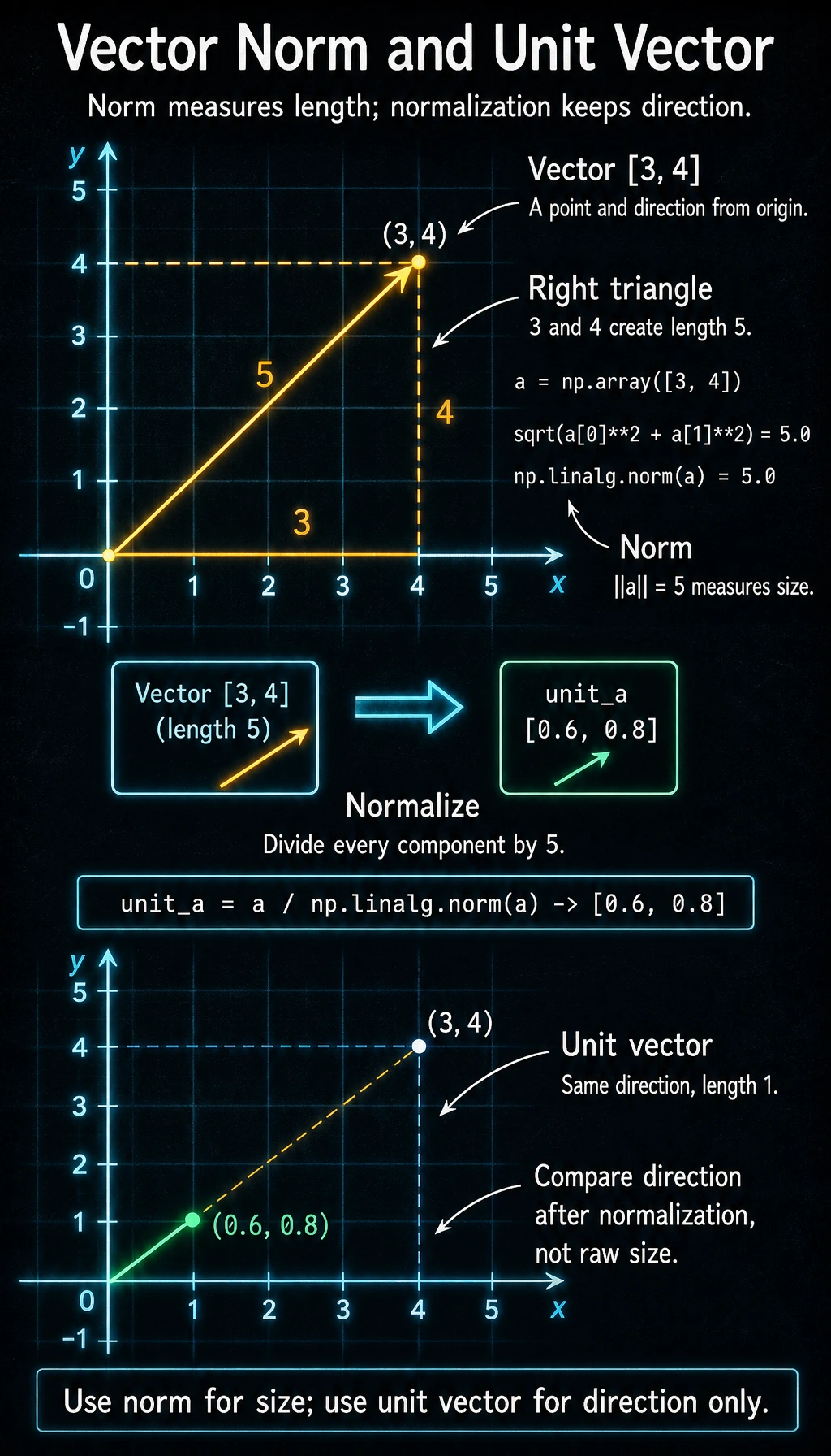
The length of a vector (also called magnitude or norm) is calculated using the Pythagorean theorem:

For vector a = [a1, a2], length = square root of (a1 squared + a2 squared)

a = np.array([3, 4])

# Method 1: manual calculation
length_manual = np.sqrt(a[0]**2 + a[1]**2)
print(f"Manual length: {length_manual}")  # 5.0

# Method 2: NumPy built-in function (recommended)
length = np.linalg.norm(a)
print(f"NumPy length: {length}")  # 5.0

The 3-4-5 triangle

The length of vector [3, 4] is exactly 5 — the classic Pythagorean triple. In data science, we will often use np.linalg.norm() to compute vector length.

Unit Vector

A vector with length 1 is called a unit vector. If you divide any vector by its length, you get a unit vector in the same direction:

a = np.array([3, 4])

# Normalize
unit_a = a / np.linalg.norm(a)
print(f"Unit vector: {unit_a}")                  # [0.6, 0.8]
print(f"Unit vector length: {np.linalg.norm(unit_a)}")  # 1.0

Why is this important? In AI, we often need to compare the direction of two vectors rather than their size. After normalization, only the directional information remains.

A Shape Sense You Must Build as a Beginner

When many people first learn vectors, they can understand the concept, but get confused by shape as soon as they write code.

import numpy as np

a = np.array([1, 2, 3])          # 1D vector
row = a.reshape(1, 3)            # row vector
col = a.reshape(3, 1)            # column vector

print("a.shape   =", a.shape)    # (3,)
print("row.shape =", row.shape)  # (1, 3)
print("col.shape =", col.shape)  # (3, 1)

They all look like “three numbers,” but in matrix multiplication they mean different things:

• (3,) is a normal 1D NumPy array
• (1, 3) explicitly means “1 row, 3 columns”
• (3, 1) explicitly means “3 rows, 1 column”

When you later learn matrices and neural networks, this shape sense is more important than memorizing formulas.

---

Dot Product — The Most Important Vector Operation

What Is the Dot Product?

The dot product of two vectors = multiply corresponding positions and then sum.

a = np.array([1, 2, 3])
b = np.array([4, 5, 6])

# Method 1: manual calculation
dot_manual = a[0]*b[0] + a[1]*b[1] + a[2]*b[2]
print(f"Manual: {dot_manual}")  # 1*4 + 2*5 + 3*6 = 32

# Method 2: NumPy (recommended)
dot_np = np.dot(a, b)
print(f"NumPy: {dot_np}")  # 32

# Method 3: @ operator (Python 3.5+)
dot_at = a @ b
print(f"@ operator: {dot_at}")  # 32

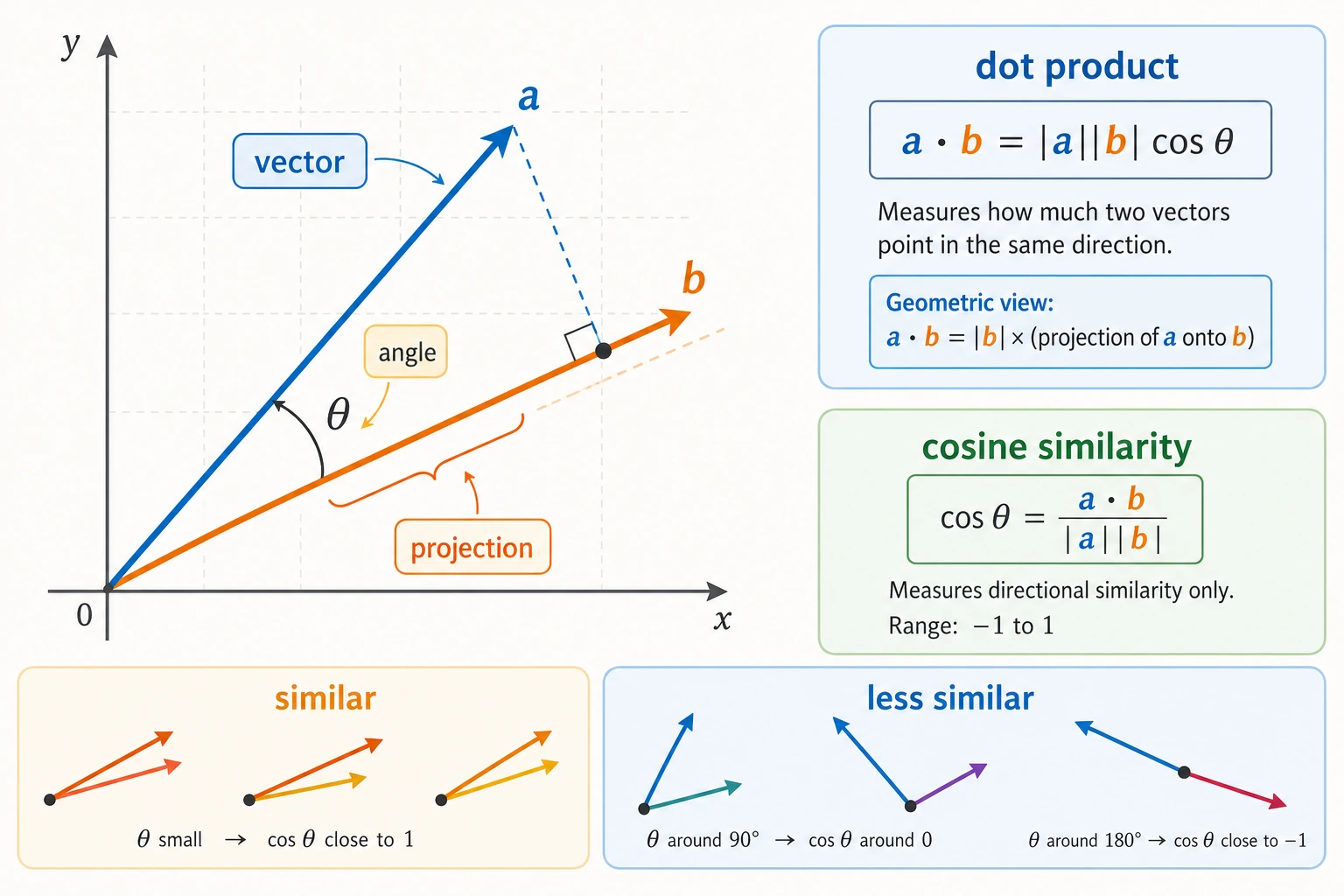
Geometric Meaning of the Dot Product

The dot product reflects the directional relationship between two vectors:

flowchart LR
    A["a · b > 0"] --> A1["Roughly the same direction<br/>angle < 90°"]
    B["a · b = 0"] --> B1["Completely perpendicular<br/>angle = 90°"]
    C["a · b < 0"] --> C1["Roughly opposite directions<br/>angle > 90°"]

    style A fill:#e8f5e9,stroke:#2e7d32,color:#333
    style B fill:#e3f2fd,stroke:#1565c0,color:#333
    style C fill:#ffebee,stroke:#c62828,color:#333

# Same direction
a = np.array([1, 0])
b = np.array([1, 1])
print(f"Same direction: a · b = {np.dot(a, b)}")  # 1 (positive)

# Perpendicular
a = np.array([1, 0])
b = np.array([0, 1])
print(f"Perpendicular: a · b = {np.dot(a, b)}")  # 0

# Opposite direction
a = np.array([1, 0])
b = np.array([-1, 0])
print(f"Opposite direction: a · b = {np.dot(a, b)}")  # -1 (negative)

Why Can the Dot Product Be Understood as “Alignment”?

The dot product can also be understood from another very important angle:

The more one vector projects onto the direction of another vector, the larger the dot product usually is.

Its formula is:

a · b = |a| × |b| × cos(theta)

You do not need to derive it first. Just remember three things for now:

1. The more two vectors point in the same direction, the closer cos(theta) is to 1
2. The more two vectors are perpendicular, the closer cos(theta) is to 0
3. The more two vectors point in opposite directions, the closer cos(theta) is to -1

So the dot product contains both:

• Length information
• Direction information

Understanding the Dot Product with Visualization

fig, axes = plt.subplots(1, 3, figsize=(15, 4))

cases = [
    ([2, 1], [1, 2], 'Same direction (dot product > 0)'),
    ([2, 0], [0, 2], 'Perpendicular (dot product = 0)'),
    ([2, 1], [-1, -2], 'Opposite direction (dot product < 0)'),
]

for ax, (a, b, title) in zip(axes, cases):
    a, b = np.array(a), np.array(b)
    dot = np.dot(a, b)

    ax.quiver(0, 0, a[0], a[1], angles='xy', scale_units='xy', scale=1,
              color='steelblue', width=0.02, label='a')
    ax.quiver(0, 0, b[0], b[1], angles='xy', scale_units='xy', scale=1,
              color='coral', width=0.02, label='b')

    ax.set_xlim(-3, 4)
    ax.set_ylim(-3, 4)
    ax.set_aspect('equal')
    ax.grid(True, alpha=0.3)
    ax.axhline(y=0, color='k', linewidth=0.5)
    ax.axvline(x=0, color='k', linewidth=0.5)
    ax.set_title(f'{title}\na·b = {dot}')
    ax.legend()

plt.tight_layout()
plt.show()

---

Cosine Similarity — The Most Common Similarity Measure in AI

From Dot Product to Cosine Similarity

The size of the dot product depends not only on direction, but also on vector length. If we only care about how similar the directions are, we need to remove the effect of length:

Cosine similarity = dot product / (length of vector A × length of vector B)

def cosine_similarity(a, b):
    """Compute the cosine similarity between two vectors"""
    dot_product = np.dot(a, b)
    norm_a = np.linalg.norm(a)
    norm_b = np.linalg.norm(b)
    if norm_a == 0 or norm_b == 0:
        raise ValueError("Cosine similarity is undefined for zero vectors.")
    return dot_product / (norm_a * norm_b)

The zero-vector check matters because a vector with length 0 has no direction. Cosine similarity compares direction, so dividing by a zero length would produce a misleading result or a runtime warning.

The range of cosine similarity is:

Value	Meaning
1	Exactly the same direction
0	Completely unrelated (perpendicular)
-1	Exactly opposite directions

Example: Runtime Profile Similarity

Suppose three model-serving profiles record five normalized signals:

# Profiles for [accuracy, throughput, low_latency, low_memory, stability] (1-5)
baseline = np.array([4, 3, 2, 2, 4])
quantized = np.array([4, 3, 3, 3, 4])
oversized = np.array([5, 1, 1, 1, 3])

# Compute pairwise similarity
print(f"Baseline vs quantized: {cosine_similarity(baseline, quantized):.4f}")
print(f"Baseline vs oversized: {cosine_similarity(baseline, oversized):.4f}")
print(f"Quantized vs oversized:{cosine_similarity(quantized, oversized):.4f}")

Output:

Baseline vs quantized: 0.9857
Baseline vs oversized: 0.9159
Quantized vs oversized:0.8775

Interpretation: the quantized model is closer to the baseline than the oversized model is to the quantized model. This is the same idea behind vector search and recommendations: compare directions first, then inspect the closest candidates with domain judgment.

Applications of Cosine Similarity in AI

flowchart TD
    CS["Cosine similarity"]
    CS --> NLP["Natural language processing<br/>word vector similarity<br/>king - man + woman ≈ queen"]
    CS --> RS["Recommendation systems<br/>user preference matching<br/>collaborative filtering"]
    CS --> RAG["RAG retrieval augmentation<br/>query-document matching<br/>vector databases"]
    CS --> IR["Image retrieval<br/>find similar images<br/>search by image"]

    style CS fill:#e3f2fd,stroke:#1565c0,color:#333
    style NLP fill:#fff3e0,stroke:#e65100,color:#333
    style RS fill:#fff3e0,stroke:#e65100,color:#333
    style RAG fill:#fff3e0,stroke:#e65100,color:#333
    style IR fill:#fff3e0,stroke:#e65100,color:#333

You will use cosine similarity again and again

• NLP (11 Natural Language Processing): compute how similar two word vectors are, for example, the cosine similarity between “cat” and “dog” is high
• RAG (8 LLM Application Development and RAG): use a vector database to retrieve the most relevant document chunks
• Recommendation systems: find users with the most similar preferences

So cosine similarity is a tool you will encounter repeatedly throughout your AI learning journey.

Visualization: Vectors with Different Cosine Similarities

fig, axes = plt.subplots(1, 4, figsize=(16, 4))

# Vector pairs with different similarities
pairs = [
    ([1, 0], [1, 0.1], '≈ 1.0 (almost identical)'),
    ([1, 0], [0.7, 0.7], '≈ 0.7 (fairly similar)'),
    ([1, 0], [0, 1], '= 0 (unrelated)'),
    ([1, 0], [-0.9, -0.3], '≈ -0.95 (opposite)'),
]

for ax, (a, b, desc) in zip(axes, pairs):
    a, b = np.array(a), np.array(b)
    sim = cosine_similarity(a, b)

    ax.quiver(0, 0, a[0], a[1], angles='xy', scale_units='xy', scale=1,
              color='steelblue', width=0.02)
    ax.quiver(0, 0, b[0], b[1], angles='xy', scale_units='xy', scale=1,
              color='coral', width=0.02)

    ax.set_xlim(-1.5, 1.5)
    ax.set_ylim(-1, 1.5)
    ax.set_aspect('equal')
    ax.grid(True, alpha=0.3)
    ax.set_title(f'cos = {sim:.2f}\n{desc}', fontsize=10)

plt.tight_layout()
plt.show()

A Minimal Retrieval Example: Find the Most Similar Item Among 3 Candidates

Although the following example uses hand-crafted small vectors, the idea is the same as vector retrieval, RAG, and semantic search.

import numpy as np

def cosine_similarity(a, b):
    return np.dot(a, b) / (np.linalg.norm(a) * np.linalg.norm(b))

query = np.array([0.9, 0.1, 0.8, 0.2])

docs = {
    "Document A: Machine Learning Basics": np.array([0.8, 0.2, 0.75, 0.1]),
    "Document B: Travel Guide":     np.array([0.1, 0.9, 0.2, 0.8]),
    "Document C: Deep Learning Basics": np.array([0.85, 0.15, 0.7, 0.25]),
}

scores = []
for name, vec in docs.items():
    sim = cosine_similarity(query, vec)
    scores.append((name, sim))

scores.sort(key=lambda x: x[1], reverse=True)

for name, sim in scores:
    print(f"{name}: {sim:.4f}")

Expected output:

Document C: Deep Learning Basics: 0.9964
Document A: Machine Learning Basics: 0.9922
Document B: Travel Guide: 0.3333

You will find that the document with the highest similarity is usually the one whose semantic direction is closest to the query.

---

NumPy Vector Operations Summary

Let’s organize all the operations learned in this section with NumPy:

import numpy as np

# ========== Create vectors ==========
a = np.array([1, 2, 3])
b = np.array([4, 5, 6])

# ========== Basic operations ==========
print("Addition:", a + b)           # [5, 7, 9]
print("Subtraction:", a - b)        # [-3, -3, -3]
print("Scalar multiplication:", 3 * a)           # [3, 6, 9]
print("Elementwise multiplication:", a * b)       # [4, 10, 18]

# ========== Dot product ==========
print("Dot product:", np.dot(a, b))    # 32
print("Dot product:", a @ b)           # 32 (equivalent)

# ========== Length (norm) ==========
print("Length:", np.linalg.norm(a))   # 3.742

# ========== Normalization ==========
unit_a = a / np.linalg.norm(a)
print("Unit vector:", unit_a)

# ========== Cosine similarity ==========
cos_sim = np.dot(a, b) / (np.linalg.norm(a) * np.linalg.norm(b))
print("Cosine similarity:", cos_sim)   # 0.9746

# scikit-learn also provides a built-in function
# from sklearn.metrics.pairwise import cosine_similarity

---

After learning this, what should you bring to the next section?

After finishing vectors, the most valuable questions to carry forward are:

1. If one object can be written as a vector, how do we write many objects at once?
2. If two vectors can be compared for similarity, how do we transform a whole batch of vectors at once?
3. Why do neural networks not process just one vector at a time, but instead always process a batch?

These three questions will naturally lead you to:

• 4.1.3 Matrices: Batch Transformations of Data

Connection to later sections

• Next section: Matrices — batch transformations for a set of vectors
• 5 Introduction to Machine Learning to Practice: in linear regression, each sample is a feature vector, and the model is finding a weight vector
• 11 Natural Language Processing (elective track): word vectors, sentence vectors, and cosine similarity appear repeatedly
• 8 LLM Application Development and RAG: the core of vector databases is similarity retrieval over high-dimensional vectors

---

Evidence to Keep

Keep this page’s proof of learning as a small evidence card:

Math Object

vector, matrix, eigenvalue, basis, or vector space concept

Numeric Example

small numbers or NumPy snippet used to compute it

Visual Or Output

shape, transformed point, similarity score, eigen direction, or projection

Ai Link

where this appears in embeddings, batches, PCA, neural layers, or attention

Expected Output

calculation plus one sentence connecting it to an AI operation

Summary

Concept	Intuitive understanding	NumPy implementation
Vector	An ordered set of numbers	np.array([1, 2, 3])
Vector addition	Add corresponding positions	a + b
Scalar multiplication	Scale the vector	k * a
Vector length	Distance from the origin to the endpoint	np.linalg.norm(a)
Dot product	Measures the directional relationship between two vectors	np.dot(a, b) or a @ b
Cosine similarity	Similarity that looks only at direction, not length	dot / (norm_a * norm_b)

What should you take away from this section?

• A vector is first of all a way to represent an object, not just an arrow
• The dot product is best understood first as “alignment”
• Cosine similarity is best understood first as “how close the directions are”
• This is why many retrieval, recommendation, and matching systems in AI cannot do without vectors

Hands-on Exercises

Exercise 1: Vector Operations

Given vectors a = [2, 3, -1] and b = [1, -2, 4], use NumPy to compute:

1. a + b
2. 3a - 2b
3. The length of a
4. The dot product of a and b
5. The cosine similarity of a and b

Exercise 2: Find the Most Similar Runtime Profile

Given three model-serving profiles:

profiles = {
    "baseline": np.array([4, 3, 2, 2, 4]),
    "quantized": np.array([4, 3, 3, 3, 4]),
    "oversized": np.array([5, 1, 1, 1, 3]),
}

Task: compute the cosine similarity between every pair of profiles, and find the closest pair and the most different pair.

Exercise 3: Visualize Vector Addition

Use Matplotlib to draw the process of the following vector addition (with arrows):

• a = [2, 3], b = [-1, 2], and draw a, b, and a+b

Hint: refer to the code in Section 2.1.

Reference implementation and walkthrough

• For a=[2,3,-1] and b=[1,-2,4], a+b=[3,1,3], 3a-2b=[4,13,-11], ||a||=sqrt(14)≈3.742, a·b=-8, and cosine similarity is about -0.8018.
• For the runtime profile vectors, the closest pair should be baseline and quantized. If you change the latency or memory dimensions, the nearest profile can change; that is the point of turning a product trade-off into numbers.
• The vector-addition plot should place a, then b from the tip of a, and show a+b=[1,5] as the final arrow from the origin. The geometry should match the numbers.