4.2.2 Probability Basics: Measuring Uncertainty

Probability distribution and Bayes update diagram

Learning Objectives

Understand the two interpretations of probability (frequentist vs. Bayesian)
Master conditional probability and joint probability
Understand Bayes’ theorem through classic examples
Use Python simulations to verify probability formulas

Terms to Decode Before the Formulas

Probability notation becomes much less scary when each symbol has a plain-language meaning:

Term	Meaning	How to read it in this lesson
`P(A)`	Probability of event A	How likely is A before knowing extra information?
`P(A\|B)`	Conditional probability	After B is known, how likely is A?
`P(A and B)`	Joint probability	How likely are A and B to happen together?
`prior`	Prior probability	What we believed before seeing new evidence
`likelihood`	Evidence probability under a hypothesis	If the hypothesis were true, how likely is this evidence?
`posterior`	Updated probability	What we believe after combining prior and evidence
`normalization`	Make probabilities sum to 1	The denominator that keeps the final answer a valid probability
`Monte Carlo`	Simulation by random sampling	Run many random trials to check whether a formula makes sense

For code in this lesson, the main dependency is NumPy. The plotting examples also use Matplotlib. To keep the examples easy to run, the joint probability table below uses only NumPy instead of adding a pandas dependency.

Historical Background: Where Did Bayes’ Rule Come From?

The most important historical milestone in this section is:

Year	Milestone	What it most importantly solved
1763	Bayes’ Theorem (later organized and published by Price)	Laid the foundation for the main line of probabilistic inference: “How do we update our judgment when new evidence appears?”

For beginners, the most important thing to remember first is not the details of the original paper, but:

The greatest value of Bayes’ rule is not the formula itself, but that it clearly explains “prior judgment + new evidence = updated judgment.”

That is also why in machine learning later on:

spam detection
medical testing
Naive Bayes

all repeatedly return to this update logic.

Why has Bayes always felt “interesting” to many beginners?

Because unlike many formulas that are just about calculation, it feels more like answering a very real-life question:

How did I originally judge this?
Now that new evidence has arrived, should I change my mind?

This is especially easy to relate to. For example, medical testing, spam detection, risk control, and recommendation systems are all essentially not about “knowing the answer absolutely,” but about:

looking at evidence
updating confidence

So the reason Bayes’ rule has been remembered for so long is often not because it is “elegant,” but because it so closely resembles how people make judgments in the real world.

Why has this been remembered by later generations?

Because it clearly told people for the first time:

reasoning does not end once you have a conclusion
reasoning can actually be updated continuously as evidence arrives

That sounds natural today, but historically it was important. You can think of Bayes’ rule as a very simple but deeply influential idea:

What I originally thought is not important; what matters is whether I am willing to update my judgment after getting new evidence.

That is why it is not just a mathematical formula, but more like an entire way of viewing an uncertain world.

First, Set a Very Important Expectation

This section will not cover everything in probability theory. Its more realistic goals are:

to help you see that “probability is not mysticism; it describes uncertainty”
to help you see that “judgments update when new information arrives”
to help you see what model output probabilities are really saying

So the most important goal in this section is not to memorize every formula perfectly, but to first clearly understand:

events
conditions
updates

These three things.

First, Build a Map

It is best to place this section back into the chapter as a whole:

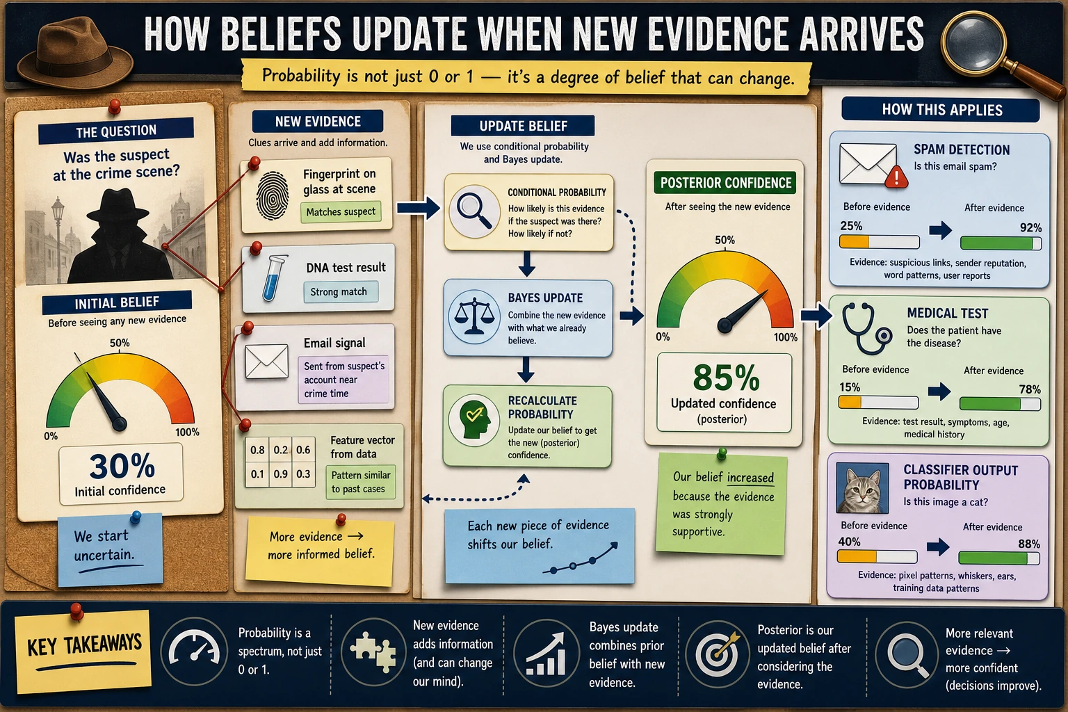
Probability and Bayes update flowchart

What you really need to learn here is not just a few formulas, but:

Many judgments in the world are not 0 or 1
When new evidence appears, our judgments are updated
This is exactly the basic idea behind AI models outputting probabilities

What Is Probability?

Two Interpretations

flowchart LR
    P["Probability"]
    P --> F["Frequentist<br/>The proportion of an event in repeated experiments<br/>Example: Flip a coin 1000 times, get heads 503 times"]
    P --> B["Bayesian<br/>The degree of confidence in an event<br/>Example: I am 80% sure it will rain tomorrow"]

    style P fill:#e3f2fd,stroke:#1565c0,color:#333
    style F fill:#fff3e0,stroke:#e65100,color:#333
    style B fill:#e8f5e9,stroke:#2e7d32,color:#333

In AI, both interpretations are used:

When training models: use frequentist methods (statistical patterns from large amounts of data)
When doing inference with models: use Bayesian methods (updating beliefs based on observations)

A More Beginner-Friendly Analogy

You can first think of probability as “confidence” in two different contexts:

Frequentist: like a statistical conclusion from repeated experiments
Bayesian: like updating your subjective confidence after getting evidence

Experiencing “Frequency Is Probability” with Python

import numpy as np
import matplotlib.pyplot as plt

plt.rcParams['font.sans-serif'] = ['Arial Unicode MS']
plt.rcParams['axes.unicode_minus'] = False

# Simulate coin flips
rng = np.random.default_rng(seed=42)
n_flips = 10000
results = rng.choice(['Heads', 'Tails'], size=n_flips)

# As the number of flips increases, the proportion of heads approaches 0.5
cumulative_ratio = np.cumsum(results == 'Heads') / np.arange(1, n_flips + 1)

plt.figure(figsize=(10, 5))
plt.plot(cumulative_ratio, color='steelblue', linewidth=1)
plt.axhline(y=0.5, color='red', linestyle='--', label='Theoretical probability 0.5')
plt.xlabel('Number of flips')
plt.ylabel('Proportion of heads')
plt.title('Law of Large Numbers: The more trials, the closer the proportion gets to the true probability')
plt.legend()
plt.xscale('log')
plt.grid(True, alpha=0.3)
plt.show()

Expected text check:

print(f"Final proportion of heads after {n_flips} flips: {cumulative_ratio[-1]:.4f}")

Example output with seed=42:

Final proportion of heads after 10000 flips: 0.5061

Law of Large Numbers: The more experiments you run, the closer the frequency gets to the true probability. This is why deep learning needs “big data.”

Conditional Probability — “Given Some Information”

Intuitive Understanding

Conditional probability P(A|B) = the probability that A happens, given that B has already happened.

Why Does Conditional Probability Feel So Much Like How AI Thinks?

Because real-world judgments almost always happen in a context.

In other words, the most important thing about conditional probability is not the symbol, but this sentence:

Once we know more information, the original judgment should be updated.

Formula and Calculation

P(A|B) = P(A and B) / P(B)

A simple intuitive example:

# A class of 100 students
# 60 like math, 50 like programming, 30 like both

n_total = 100
n_math = 60
n_code = 50
n_both = 30

# P(like programming | like math) = P(like both) / P(like math)
p_code_given_math = n_both / n_math
print(f"Among students who like math, the proportion who also like programming: {p_code_given_math:.1%}")  # 50%

# P(like math | like programming)
p_math_given_code = n_both / n_code
print(f"Among students who like programming, the proportion who also like math: {p_math_given_code:.1%}")  # 60%

Expected output:

Among students who like math, the proportion who also like programming: 50.0%
Among students who like programming, the proportion who also like math: 60.0%

Note: P(A|B) and P(B|A) are usually not equal!

This Is One of the Easiest Pitfalls for Beginners

When many people first learn this, they instinctively mix up:

“Among people who like math, how many like programming”

with

“Among people who like programming, how many like math”

But they have different denominators, so they are fundamentally different questions.

Joint Probability and Marginal Probability

# Simulate data with NumPy
rng = np.random.default_rng(seed=42)
n = 10000

# Service state: healthy (0.85) / degraded (0.15)
service_state = rng.choice(['Healthy', 'Degraded'], n, p=[0.85, 0.15])

# Alert probability depends on service state
alert = np.where(
    service_state == 'Degraded',
    rng.choice(['Alert', 'No alert'], n, p=[0.75, 0.25]),  # 75% alert when degraded
    rng.choice(['Alert', 'No alert'], n, p=[0.05, 0.95])   # 5% alert when healthy
)

# Joint probability table without extra dependencies
state_labels = ['Healthy', 'Degraded']
alert_labels = ['Alert', 'No alert']
joint = np.array([
    [((service_state == s) & (alert == a)).mean() for a in alert_labels]
    for s in state_labels
])

print("Joint probability table:")
print("             Alert  No alert")
for label, row in zip(state_labels, joint):
    print(f"{label:>9}   {row[0]:.3f}    {row[1]:.3f}")
print(f"\nMarginal probability P(degraded): {(service_state == 'Degraded').mean():.3f}")
print(f"Marginal probability P(alert): {(alert == 'Alert').mean():.3f}")

Expected output with seed=42:

Joint probability table:
             Alert  No alert
  Healthy   0.043    0.809
 Degraded   0.109    0.039

Marginal probability P(degraded): 0.147
Marginal probability P(alert): 0.152

	Alert	No alert	Total (marginal probability)
Healthy	0.04	0.81	0.85
Degraded	0.11	0.04	0.15
Total	0.15	0.85	1.00

The table is slightly different from the ideal values because it is simulated. With more samples, it will get closer to the theoretical table.

Bayes’ Theorem — The Most Important Probability Formula in AI

Introduction: The Story of a Hospital Test

A rare disease has an incidence rate of 0.1% (1 in 1000 people has it). A hospital has a test:

If you have the disease, the probability the test is positive is 99% (sensitivity)
If you do not have the disease, the probability the test is positive is 5% (false positive rate)

Question: If your test comes back positive, what is the probability that you really have the disease?

Many people instinctively say “99%” — but the answer may surprise you.

Bayes’ Formula

P(Have disease | Positive) = P(Positive | Have disease) × P(Have disease) / P(Positive)

# Given conditions
p_disease = 0.001       # Prior probability: incidence rate 0.1%
p_positive_if_disease = 0.99    # Have disease → probability of positive
p_positive_if_healthy = 0.05    # No disease → probability of positive (false positive rate)

# P(Positive) = P(Positive|Have disease)×P(Have disease) + P(Positive|No disease)×P(No disease)
p_positive = (p_positive_if_disease * p_disease +
              p_positive_if_healthy * (1 - p_disease))
print(f"P(Positive): {p_positive:.4f}")

# Bayes' formula
p_disease_if_positive = (p_positive_if_disease * p_disease) / p_positive
print(f"P(Have disease|Positive): {p_disease_if_positive:.4f}")  # ≈ 0.0194
print(f"Approximately {p_disease_if_positive:.1%}")             # ≈ 1.9%

Expected output:

P(Positive): 0.0509
P(Have disease|Positive): 0.0194
Approximately 1.9%

Result: only about 2%! Even if the test is positive, the probability that you actually have the disease is only 2%.

Why Is It So Low?

Because the incidence rate is too low (0.1%), most positive results are actually false positives.

# Simulate with 10000 people
n_people = 10000
n_sick = int(n_people * p_disease)        # 10 people have the disease
n_healthy = n_people - n_sick             # 9990 people do not have the disease

true_positive = n_sick * p_positive_if_disease    # have disease and test positive: ≈ 10
false_positive = n_healthy * p_positive_if_healthy # no disease but test positive: ≈ 500

total_positive = true_positive + false_positive

print(f"Out of 10000 people:")
print(f"  People with the disease: {n_sick}")
print(f"  People who test positive: {total_positive:.0f}")
print(f"    Of which true positives: {true_positive:.0f}")
print(f"    Of which false positives: {false_positive:.0f}")
print(f"  Proportion of truly sick among positive results: {true_positive/total_positive:.1%}")

Expected output:

Out of 10000 people:
  People with the disease: 10
  People who test positive: 509
    Of which true positives: 10
    Of which false positives: 500
  Proportion of truly sick among positive results: 1.9%

flowchart TD
    A["10000 people"] --> B["10 people have the disease"]
    A --> C["9990 people do not have the disease"]
    B --> D["≈ 10 people test positive<br/>(true positives)"]
    C --> E["≈ 500 people test positive<br/>(false positives)"]
    D --> F["Total positives ≈ 510<br/>Only 10 are truly sick<br/>≈ 2%"]
    E --> F

    style D fill:#e8f5e9,stroke:#2e7d32,color:#333
    style E fill:#ffebee,stroke:#c62828,color:#333
    style F fill:#fff3e0,stroke:#e65100,color:#333

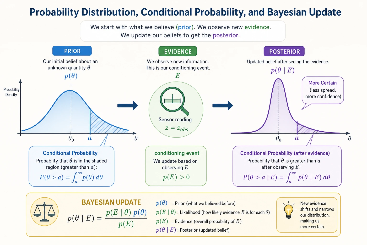
The Core Idea of Bayes’ Theorem

flowchart LR
    A["Prior P(A)<br/>Belief before evidence"] -->|"See evidence B"| B["Posterior P(A|B)<br/>Updated belief"]
    C["Likelihood P(B|A)<br/>How strongly the evidence supports it"] --> B

    style A fill:#e3f2fd,stroke:#1565c0,color:#333
    style B fill:#e8f5e9,stroke:#2e7d32,color:#333
    style C fill:#fff3e0,stroke:#e65100,color:#333

Posterior = Prior × Likelihood / Normalization factor

This is the core of Bayes: continuously updating your belief with new evidence.

Verifying Bayes’ Theorem with Simulation

# Monte Carlo simulation
rng = np.random.default_rng(seed=42)
n_sim = 1_000_000

# 1. Whether each person has the disease
has_disease = rng.random(n_sim) < p_disease

# 2. Each person's test result
test_positive = np.where(
    has_disease,
    rng.random(n_sim) < p_positive_if_disease,  # Have disease
    rng.random(n_sim) < p_positive_if_healthy    # No disease
)

# 3. Among those who test positive, the proportion who are sick
positive_people = test_positive.sum()
positive_and_sick = (test_positive & has_disease).sum()

simulated_probability = positive_and_sick / positive_people
print(f"Simulated result P(Have disease|Positive): {simulated_probability:.4f}")
print(f"Formula result: {p_disease_if_positive:.4f}")
print(f"Difference: {abs(simulated_probability - p_disease_if_positive):.6f}")

Expected output with seed=42:

Simulated result P(Have disease|Positive): 0.0194
Formula result: 0.0194
Difference: 0.000012

Simulation is not a replacement for the formula. It is a learning tool: it helps you see that the formula matches what happens after many random trials.

Applications of Bayes’ Theorem in AI

Naive Bayes Classifier

Spam filtering is a classic application of Bayes’ theorem:

# Simplified spam classification
# P(Spam | contains "free") = P(contains "free"|Spam) × P(Spam) / P(contains "free")

p_spam = 0.3                      # 30% of emails are spam
p_free_given_spam = 0.8           # 80% of spam emails contain "free"
p_free_given_ham = 0.05           # 5% of normal emails contain "free"

# P(contains "free")
p_free = p_free_given_spam * p_spam + p_free_given_ham * (1 - p_spam)

# Bayes
p_spam_given_free = p_free_given_spam * p_spam / p_free
print(f"Probability that an email containing 'free' is spam: {p_spam_given_free:.1%}")
# ≈ 87.3%

Expected output:

Probability that an email containing 'free' is spam: 87.3%

More AI Applications

Application	Prior	Likelihood	Posterior
Spam filtering	Probability that an email is spam	Probability that spam contains a certain word	Probability that it is spam given the word
Medical diagnosis	Incidence rate of a disease	Probability of a positive test when diseased	Probability of truly being sick after a positive result
Model routing	Probability that a request needs a stronger model	Probability that similar hard requests failed on a small model	Probability that this request should be routed up
Language models	Probability of a word appearing	Probability that the word appears given the context	Most likely next word

Independence — A Powerful Tool for Simplifying Calculations

What Is Independence?

Two events are independent, meaning the occurrence of one does not affect the probability of the other.

P(A and B) = P(A) × P(B) (only when A and B are independent)

# Flipping two coins — the two flips are independent
p_head = 0.5

# Both are heads
p_both_heads = p_head * p_head
print(f"Both flips are heads: {p_both_heads}")  # 0.25

# Simulation check
rng = np.random.default_rng(seed=42)
n = 100000
coin1 = rng.random(n) < 0.5
coin2 = rng.random(n) < 0.5
both = (coin1 & coin2).mean()
print(f"Simulated result: {both:.4f}")  # ≈ 0.25

Expected output:

Both flips are heads: 0.25
Simulated result: 0.2512

The Independence Assumption in AI

Naive Bayes is called “naive” because it assumes all features are independent (although in reality they often are not, the method still works surprisingly well).

This assumption is not literally true for natural language. For example, “free” and “winner” often appear together in spam. But the assumption makes the calculation much simpler, and the simplified model is often good enough as a baseline. A baseline is a simple first model used to check whether more complex methods are truly improving things.

# Naive Bayes: assume each word appears independently
# P(Spam|"free","winner","click") ∝ P(Spam) × P("free"|Spam) × P("winner"|Spam) × P("click"|Spam)

p_spam = 0.3
words = {
    "free": (0.8, 0.05),    # (P(word|spam), P(word|normal))
    "winner": (0.6, 0.01),
    "click": (0.7, 0.1),
}

# Compute numerator
score_spam = p_spam
score_ham = 1 - p_spam

for word, (p_word_spam, p_word_ham) in words.items():
    score_spam *= p_word_spam
    score_ham *= p_word_ham

# Normalize
p_spam_given_words = score_spam / (score_spam + score_ham)
print(f"Probability that an email containing 'free' + 'winner' + 'click' is spam: {p_spam_given_words:.1%}")

Expected output:

Probability that an email containing 'free' + 'winner' + 'click' is spam: 100.0%

The result is extremely close to 100% because the example probabilities are intentionally exaggerated for teaching. In real systems, you would usually apply smoothing, evaluate on held-out data, and avoid treating one output as absolute truth.

After Learning This, What Should You Bring to the Next Section?

After finishing probability basics, the most worthwhile questions to carry forward are:

If a single event can be described by probability, what will a collection of many random outcomes look like overall?
Why do some phenomena always seem like bell curves, while others look more like count distributions?
Why are noise, initialization, and errors in models so often tied to certain distributions?

These three questions will naturally lead you to:

4.2.3 Probability Distributions: Patterns Behind Data

Evidence to Keep

Keep this page’s proof of learning as a small evidence card:

Random Process: event, distribution, sample, likelihood, entropy, or Bayes update
Simulation Or Formula: code or formula used to make uncertainty visible
Output: probability, sample statistic, interval, entropy, or updated belief
Failure Check: base-rate confusion, p-value misuse, sample bias, or mixing probability with certainty
Expected Output: numeric result plus interpretation in plain language

Summary

Concept	Intuition	Formula / Code
Probability	A measure of uncertainty (0~1)	`rng.random() < p`
Conditional probability	Probability of A given B has occurred	P(A\|B) = P(A and B) / P(B)
Joint probability	Probability of A and B happening together	NumPy boolean masks such as `(A & B).mean()`
Bayes’ theorem	Updating beliefs with evidence	Posterior = Prior × Likelihood / Normalization
Independence	No mutual influence	P(A and B) = P(A) × P(B)

What Should You Take Away from This Section?

Probability describes uncertainty; it does not pretend things are absolutely certain
The most important intuition for conditional probability is: “when information changes, the judgment should change too”
The most important thing to remember about Bayes is: “prior + evidence -> updated judgment”
That is why many outputs in AI are naturally probabilities, not absolute conclusions

Hands-on Exercises

Exercise 1: Conditional Probability

From a standard 52-card deck, draw one card at random:

P(hearts) = ?
P(hearts | red card) = ? (given that it is a red card)
P(A | hearts) = ? (given that it is a heart)

Use Python to simulate and verify 100000 trials.

Reference implementation:

rng = np.random.default_rng(seed=42)
n_trials = 100000

suits = np.array(['hearts', 'diamonds', 'clubs', 'spades'])
ranks = np.array(['A', '2', '3', '4', '5', '6', '7', '8', '9', '10', 'J', 'Q', 'K'])
deck = [(suit, rank) for suit in suits for rank in ranks]

indices = rng.integers(0, len(deck), size=n_trials)
draws = [deck[i] for i in indices]

is_hearts = np.array([suit == 'hearts' for suit, rank in draws])
is_red = np.array([suit in {'hearts', 'diamonds'} for suit, rank in draws])
is_ace = np.array([rank == 'A' for suit, rank in draws])

print(f"P(hearts): {is_hearts.mean():.3f}")
print(f"P(hearts | red): {(is_hearts & is_red).sum() / is_red.sum():.3f}")
print(f"P(A | hearts): {(is_ace & is_hearts).sum() / is_hearts.sum():.3f}")

Expected output with seed=42:

P(hearts): 0.250
P(hearts | red): 0.501
P(A | hearts): 0.076

Exercise 2: Bayes Update

A factory has two production lines, A and B. Line A produces 60% of the products, and line B produces 40%. The defect rate of A is 2%, and the defect rate of B is 5%.

If a randomly selected product is found to be defective, what is the probability that it came from production line B?

Reference implementation:

p_a = 0.6
p_b = 0.4
p_defective_given_a = 0.02
p_defective_given_b = 0.05

p_defective = p_defective_given_a * p_a + p_defective_given_b * p_b
p_b_given_defective = p_defective_given_b * p_b / p_defective

print(f"P(line B | defective): {p_b_given_defective:.1%}")

Expected output:

P(line B | defective): 62.5%

Exercise 3: Simulate Bayes’ Theorem

Modify the disease testing example by changing the incidence rate to 1% (instead of 0.1%), and see how the probability of having the disease after a positive test changes. Verify it using both simulation and the formula.

Formula check:

p_disease = 0.01
p_positive_if_disease = 0.99
p_positive_if_healthy = 0.05

p_positive = (p_positive_if_disease * p_disease +
              p_positive_if_healthy * (1 - p_disease))
p_disease_if_positive = p_positive_if_disease * p_disease / p_positive

print(f"P(Have disease|Positive) when incidence is 1%: {p_disease_if_positive:.1%}")

Expected output:

P(Have disease|Positive) when incidence is 1%: 16.7%

This is much higher than 1.9%, because the prior probability is no longer as tiny. Bayes’ theorem is sensitive to the prior, which is exactly why base rates matter so much in real-world diagnosis and risk scoring.

Operation guide and checkpoints

For the card problem, P(hearts)=13/52=0.25, P(hearts | red)=13/26=0.5, and P(A | hearts)=1/13≈0.0769. Simulation should be close, not exact.
For the factory Bayes problem, P(defective)=0.6*0.02+0.4*0.05=0.032, so P(B | defective)=0.02/0.032=62.5%.
If disease incidence changes from 0.1% to 1%, the posterior after a positive test rises sharply. That is the main lesson: base rate changes the meaning of the same test result.