3.2.6 Basic Linear Algebra Operations

Learning Objectives

• Master three ways to write matrix multiplication (dot, matmul, @)
• Understand the meaning and computation of inverse matrices, determinants, and eigenvalues
• Learn to use the numpy.linalg module for linear algebra operations
• Understand why linear algebra matters in AI

---

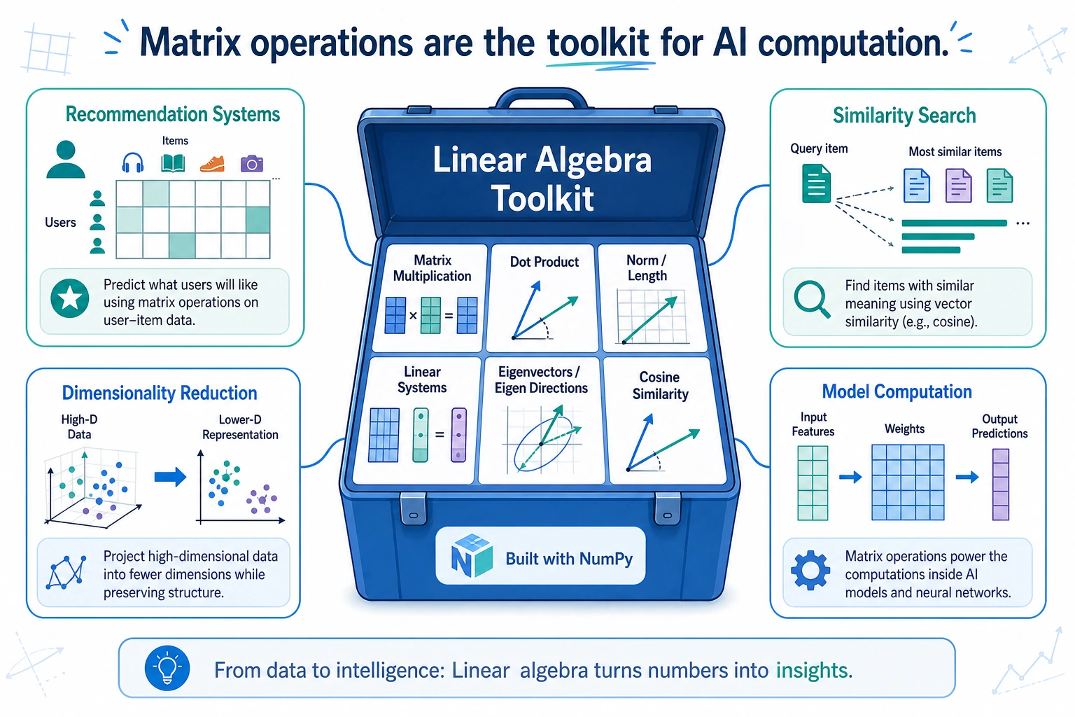
Why learn linear algebra?

You may feel that “linear algebra” sounds very mathematical and abstract. But in AI, it is one of the most essential mathematical foundations:

AI Scenario	Role of Linear Algebra
Neural networks	The computation in each layer is matrix multiplication
Recommender systems	User-item matrix factorization
Image processing	An image is a matrix
Word vectors	Each word is a vector; similarity = dot product
Dimensionality reduction	PCA is about finding eigenvalues and eigenvectors

For now, let’s use NumPy to work with these concepts and build intuition. Chapter 4, The Minimum Necessary Math Foundation for AI, will explain the principles in more depth.

---

Matrix multiplication

Element-wise multiplication vs. matrix multiplication

This is one of the most common points of confusion for beginners:

import numpy as np

A = np.array([[1, 2], [3, 4]])
B = np.array([[5, 6], [7, 8]])

# Element-wise multiplication
print(A * B)
# [[ 5 12]
#  [21 32]]
# Calculation: 1×5=5, 2×6=12, 3×7=21, 4×8=32

# Matrix multiplication
print(A @ B)
# [[19 22]
#  [43 50]]
# Calculation:
# [1×5+2×7, 1×6+2×8]   = [19, 22]
# [3×5+4×7, 3×6+4×8]   = [43, 50]

Three ways to write matrix multiplication

A = np.array([[1, 2], [3, 4]])
B = np.array([[5, 6], [7, 8]])

# Method 1: @ operator (recommended, most concise)
C1 = A @ B

# Method 2: np.matmul
C2 = np.matmul(A, B)

# Method 3: np.dot
C3 = np.dot(A, B)

# All three methods give exactly the same result
print(np.array_equal(C1, C2))  # True
print(np.array_equal(C2, C3))  # True

Use @

In Python 3.5+, the @ operator is the most recommended way to write matrix multiplication because it is concise and intuitive.

Rules for matrix multiplication

Two matrices can be multiplied only when: the number of columns in the first matrix = the number of rows in the second matrix.

# (2, 3) @ (3, 4) → (2, 4)  ✅ 3 == 3
A = np.ones((2, 3))
B = np.ones((3, 4))
C = A @ B
print(C.shape)   # (2, 4)

# (2, 3) @ (2, 4) → ❌ error! 3 ≠ 2
# A = np.ones((2, 3))
# B = np.ones((2, 4))
# C = A @ B  # ValueError!

Memory trick: (m, n) @ (n, p) → (m, p)

Vector dot product

For one-dimensional arrays, @ or np.dot computes the dot product:

a = np.array([1, 2, 3])
b = np.array([4, 5, 6])

# Dot product = 1×4 + 2×5 + 3×6 = 32
print(a @ b)        # 32
print(np.dot(a, b)) # 32

The dot product is very important in AI—you will use it later when learning cosine similarity and the attention mechanism.

---

The numpy.linalg module

NumPy’s linalg submodule provides a full set of linear algebra functions:

Inverse matrix

The inverse of a matrix satisfies A × A⁻¹ = identity matrix:

A = np.array([[1, 2], [3, 4]])

# Compute the inverse matrix
A_inv = np.linalg.inv(A)
print(A_inv)
# [[-2.   1. ]
#  [ 1.5 -0.5]]

# Verify: A × A_inv ≈ identity matrix
print(A @ A_inv)
# [[1.0000000e+00 0.0000000e+00]
#  [8.8817842e-16 1.0000000e+00]]
# The diagonal is 1, and the other values are close to 0 (floating-point precision error)

Not every matrix has an inverse

Only square matrices (same number of rows and columns) with non-zero determinant have an inverse.

# A singular matrix (determinant = 0) has no inverse
singular = np.array([[1, 2], [2, 4]])  # The second row is 2 times the first row
# np.linalg.inv(singular)  # LinAlgError: Singular matrix

Determinant

The determinant is a scalar value that represents the matrix’s “scaling factor”:

A = np.array([[1, 2], [3, 4]])
det = np.linalg.det(A)
print(f"Determinant: {det:.1f}")   # -2.0

# Determinant of a 2×2 matrix = ad - bc
# [[a, b], [c, d]] → 1×4 - 2×3 = -2

Eigenvalues and eigenvectors

Eigenvalues and eigenvectors are the “DNA” of a matrix—they reveal its internal properties:

A = np.array([[4, 2], [1, 3]])

# Compute eigenvalues and eigenvectors
eigenvalues, eigenvectors = np.linalg.eig(A)
print(f"Eigenvalues: {eigenvalues}")      # [5. 2.]
print(f"Eigenvectors:\n{eigenvectors}")
# [[ 0.894 -0.707]
#  [ 0.447  0.707]]

Intuition for eigenvalues

If you think of a matrix as a kind of “transformation” (such as rotation or stretching), then:

• Eigenvectors = vectors whose direction does not change after the transformation
• Eigenvalues = the amount of stretching along that direction

This concept will be very useful later when we learn PCA for dimensionality reduction—PCA is essentially about finding the directions where the data changes the most (the eigenvectors corresponding to the largest eigenvalues).

Solving systems of linear equations

Solve the equations:
2x + y = 5
x + 3y = 7

Write them in matrix form: Ax = b

A = np.array([[2, 1], [1, 3]])
b = np.array([5, 7])

# Solve the system
x = np.linalg.solve(A, b)
print(f"x = {x[0]:.2f}, y = {x[1]:.2f}")  # x = 1.60, y = 1.80

# Verify
print(A @ x)   # [5. 7.]  ← equals b, so the solution is correct

---

Other useful operations

Norms (vector length)

v = np.array([3, 4])

# L2 norm (Euclidean distance)
l2 = np.linalg.norm(v)
print(f"L2 norm: {l2}")   # 5.0  (3² + 4² = 25, √25 = 5)

# L1 norm (sum of absolute values)
l1 = np.linalg.norm(v, ord=1)
print(f"L1 norm: {l1}")   # 7.0  (|3| + |4| = 7)

# Matrix norm
M = np.array([[1, 2], [3, 4]])
print(f"Matrix Frobenius norm: {np.linalg.norm(M):.2f}")  # 5.48

Matrix rank

A = np.array([[1, 2, 3], [4, 5, 6], [7, 8, 9]])
rank = np.linalg.matrix_rank(A)
print(f"Matrix rank: {rank}")  # 2 (not full rank, because the third row = first row×(-1) + second row×2)

Quick reference for common functions

Function	Purpose	Example
A @ B	Matrix multiplication	np.array([[1,2],[3,4]]) @ np.eye(2)
np.linalg.inv(A)	Inverse matrix
np.linalg.det(A)	Determinant
np.linalg.eig(A)	Eigenvalues and eigenvectors
np.linalg.solve(A, b)	Solve Ax=b
np.linalg.norm(v)	Norm
np.linalg.matrix_rank(A)	Matrix rank
A.T	Transpose
np.trace(A)	Trace (sum of diagonal elements)

---

Practice: Calculate cosine similarity

Cosine similarity is a common way in AI to measure how “similar” two vectors are. It will be used repeatedly later in word vectors, recommender systems, and RAG.

Formula: cos(θ) = (a · b) / (||a|| × ||b||)

import numpy as np

def cosine_similarity(a, b):
    """Calculate the cosine similarity between two vectors"""
    dot_product = a @ b                         # Dot product
    norm_a = np.linalg.norm(a)                  # Length of a
    norm_b = np.linalg.norm(b)                  # Length of b
    return dot_product / (norm_a * norm_b)

# Example: compare model-serving profiles
# Dimensions represent: [accuracy, throughput, low_latency, low_memory, stability]
baseline = np.array([4, 3, 2, 2, 4])
quantized = np.array([4, 3, 3, 3, 4])
experimental = np.array([2, 5, 5, 4, 2])

print(f"Baseline vs quantized: {cosine_similarity(baseline, quantized):.4f}")      # 0.9857
print(f"Baseline vs experimental: {cosine_similarity(baseline, experimental):.4f}")  # 0.8137
print(f"Quantized vs experimental: {cosine_similarity(quantized, experimental):.4f}") # 0.8778

---

Evidence to Keep

Keep this page’s proof of learning as a small evidence card:

Array State

shape, dtype, axis, and sample values before the operation

Operation

indexing, slicing, broadcasting, reshape, linear algebra, or random/stat function

Output

resulting array shape, values, or statistic

Failure Check

axis confusion, view/copy trap, broadcast mismatch, or wrong shape

Expected Output

printed shapes and values that make the array operation inspectable

Summary

Concept	Description	NumPy function
Matrix multiplication	(m,n) @ (n,p) → (m,p)	A @ B or np.matmul
Inverse matrix	A × A⁻¹ = I	np.linalg.inv()
Determinant	Matrix scaling factor	np.linalg.det()
Eigenvalues/vectors	The “DNA” of a matrix	np.linalg.eig()
Solving equations	Solve Ax = b	np.linalg.solve()
Norm	Vector length	np.linalg.norm()

How much do you need to learn?

At this stage, you only need to:

1. Be able to use NumPy’s linear algebra functions
2. Know roughly what matrix multiplication, inverse matrices, and eigenvalues mean
3. Be able to calculate cosine similarity

You will learn the deeper mathematical understanding systematically in Chapter 4, The Minimum Necessary Math Foundation for AI. For now, just build intuition through code.

---

Hands-on exercises

Exercise 1: Matrix multiplication

# Resource cost per request for 3 pipeline stages
cost_per_stage = np.array([4, 12, 6])   # [embed, rerank, generate]

# Stage counts for 3 request batches
stage_counts = np.array([
    [3, 1, 2],    # Batch 1
    [0, 2, 5],    # Batch 2
    [5, 0, 3]     # Batch 3
])

# Use matrix multiplication to calculate the total cost of each batch
# totals = ?

Exercise 2: Solve equations

# Solve the system:
# 3x + 2y - z = 1
# x - y + 2z = 5
# 2x + 3y - z = 0
#
# Hint: write it in the form Ax = b

Exercise 3: Cosine similarity application

# Suppose we have feature vectors for model-serving profiles
# Dimensions represent: [accuracy, throughput, low_latency, low_memory, stability]
profiles = {
    "baseline": np.array([4, 3, 2, 2, 4]),
    "quantized": np.array([4, 3, 3, 3, 4]),
    "experimental": np.array([2, 5, 5, 4, 2]),
}

# Use cosine similarity to find the profile most similar to "baseline"
# Hint: calculate the cosine similarity between "baseline" and each other profile

Reference implementation and walkthrough

• For the resource-cost example, stage_counts @ cost_per_stage is the clean vectorized answer. With costs [4, 12, 6] and rows [3,1,2], [0,2,5], [5,0,3], the totals are 36, 54, and 38.
• For the linear system 3x + 2y - z = 1, x - y + 2z = 5, 2x + 3y - z = 0, np.linalg.solve should return x=1, y=0, z=2.
• In the profile cosine-similarity example, compare dot products after normalizing by vector length. The most similar profile should be the one with the largest cosine value, not simply the largest raw dot product.