6.6.3 VAE Basics [Optional]

Learning Objectives

Explain the encoder, mu, logvar, latent sample z, and decoder.
Understand why VAE uses reparameterization.
Run a tiny PyTorch VAE on 2D points.
Read reconstruction loss and KL regularization.
Compare VAE with a standard autoencoder and GAN.

See the Flow First

VAE latent space generation flowchart

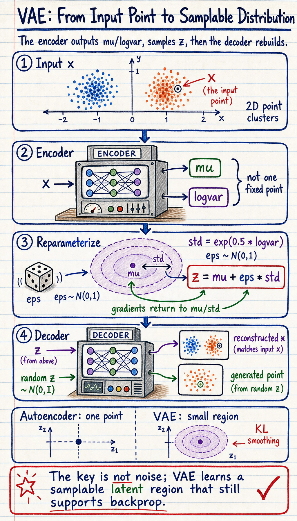
Step	What happens	Practical meaning
Encode	`x -> mu, logvar`	describe a latent region
Sample	`z = mu + eps * std`	make sampling differentiable
Decode	`z -> reconstructed x`	turn latent code back into data
Regularize	KL term	keep latent space smooth and samplable

The key difference from a normal autoencoder:

Autoencoder: x -> one latent point -> reconstruction
VAE: x -> latent distribution -> sample z -> reconstruction or generation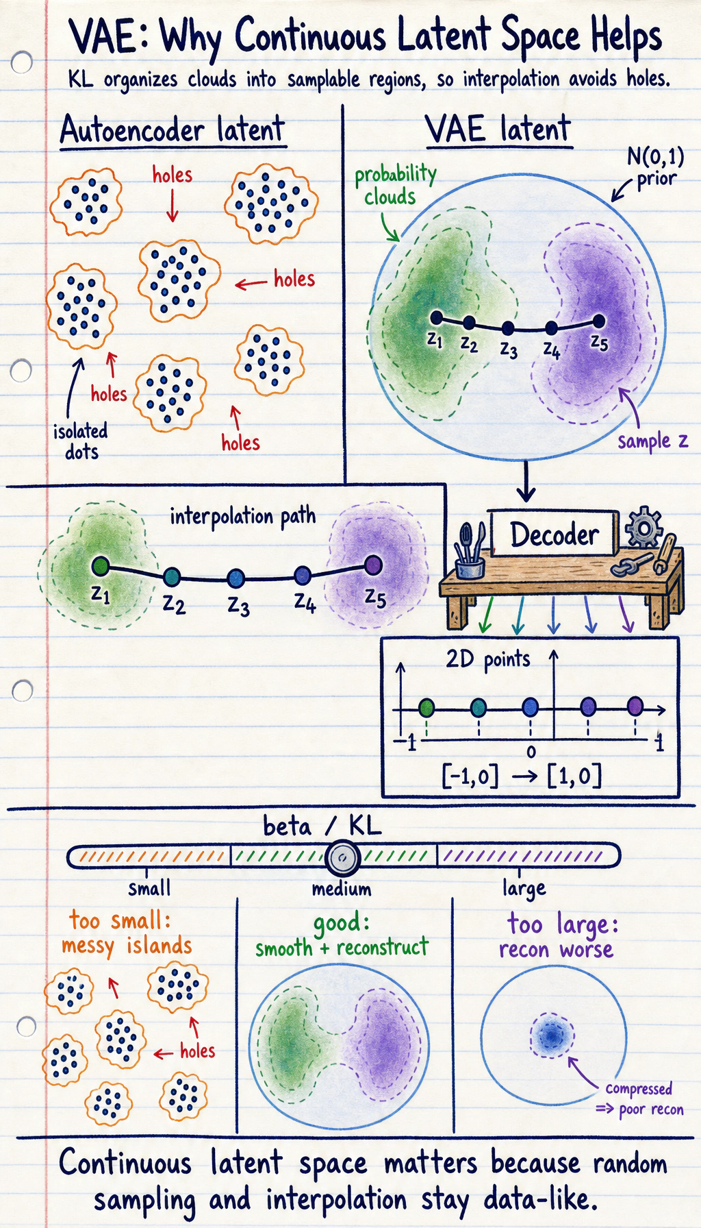

VAE continuous latent space and sampling region diagram

Why Reparameterization Exists

Sampling is random. Random sampling by itself blocks straightforward backpropagation. VAE rewrites sampling as:

std = exp(0.5 * logvar)
eps ~ N(0, 1)
z = mu + eps * std

Now gradients can flow through mu and std, while eps provides randomness.

The VAE Loss

VAE training usually combines two goals:

loss = reconstruction_loss + beta * KL(q(z|x) || p(z))

Read it in plain language:

reconstruction loss: “can the decoder rebuild the input?”
KL term: “is the latent space close to a smooth prior such as N(0, 1)?”
beta: how strongly you force the latent space to be regular.

Too little KL pressure can make the latent space messy. Too much KL pressure can hurt reconstruction or cause the latent variable to carry too little information.

Lab: Train a Tiny VAE on 2D Points

This is not an image VAE. It is a small runnable lab that exposes the full mechanics.

Create tiny_vae_2d.py:

import torch
from torch import nn

torch.manual_seed(4)

cluster_a = torch.randn(128, 2) * 0.15 + torch.tensor([1.0, 0.0])
cluster_b = torch.randn(128, 2) * 0.15 + torch.tensor([-1.0, 0.0])
x = torch.cat([cluster_a, cluster_b], dim=0)


class TinyVAE(nn.Module):
    def __init__(self):
        super().__init__()
        self.encoder = nn.Sequential(nn.Linear(2, 16), nn.ReLU())
        self.mu = nn.Linear(16, 2)
        self.logvar = nn.Linear(16, 2)
        self.decoder = nn.Sequential(nn.Linear(2, 16), nn.ReLU(), nn.Linear(16, 2))

    def reparameterize(self, mu, logvar):
        std = torch.exp(0.5 * logvar)
        eps = torch.randn_like(std)
        return mu + eps * std

    def forward(self, x):
        h = self.encoder(x)
        mu = self.mu(h)
        logvar = self.logvar(h)
        z = self.reparameterize(mu, logvar)
        recon = self.decoder(z)
        return recon, mu, logvar


model = TinyVAE()
opt = torch.optim.Adam(model.parameters(), lr=0.02)

for epoch in range(1, 201):
    recon, mu, logvar = model(x)
    recon_loss = ((recon - x) ** 2).mean()
    kl = -0.5 * torch.mean(1 + logvar - mu.pow(2) - logvar.exp())
    loss = recon_loss + 0.05 * kl

    opt.zero_grad()
    loss.backward()
    opt.step()

    if epoch in [1, 50, 100, 200]:
        print(
            f"epoch={epoch:03d} "
            f"recon={recon_loss.item():.4f} "
            f"kl={kl.item():.4f} "
            f"loss={loss.item():.4f}"
        )

with torch.no_grad():
    z = torch.randn(5, 2)
    samples = model.decoder(z)
    rounded = [[round(v, 3) for v in row.tolist()] for row in samples]
    print("generated_points")
    print(rounded)

Run it:

python tiny_vae_2d.py

Expected output:

epoch=001 recon=0.5903 kl=0.0293 loss=0.5917
epoch=050 recon=0.0335 kl=0.9007 loss=0.0785
epoch=100 recon=0.0261 kl=0.8229 loss=0.0673
epoch=200 recon=0.0244 kl=0.7138 loss=0.0601
generated_points
[[1.075, -0.014], [-0.997, -0.001], [-1.118, -0.054], [0.553, 0.041], [0.74, 0.021]]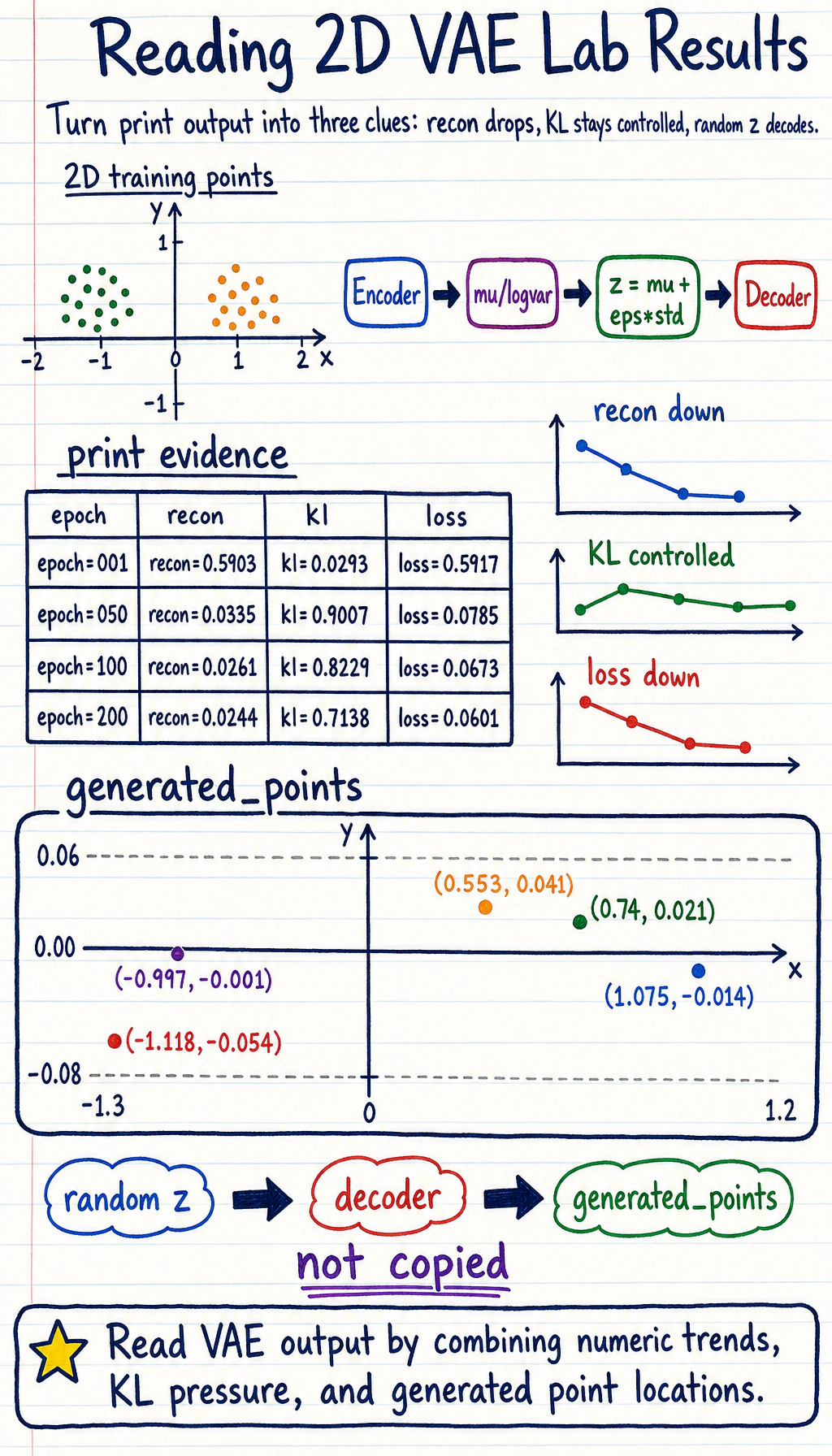

2D VAE lab result map

Read the output:

recon drops when the decoder learns to rebuild the 2D points.
kl does not need to become zero. It is a pressure toward a smooth latent prior.
generated_points are decoded from random z, not copied directly from training data.

Evidence to Keep

For a VAE run, keep this record:

Recon Trend: reconstruction loss decreases
Kl Trend: KL stays nonzero but controlled
Sample Check: generated_points come from random z
Tradeoff: better reconstruction <→ smoother latent space
Next Probe: change KL weight and compare samples

This evidence is what separates a VAE from a plain autoencoder: the latent space should be usable for sampling, not only reconstruction.

VAE vs Autoencoder vs GAN

Model	Learns	Strength	Typical weakness
Autoencoder	compact representation	reconstruction	latent space may not be easy to sample
VAE	distribution-shaped latent space	smooth sampling and interpolation	output can be blurry in image tasks
GAN	adversarial realism	sharp-looking samples	unstable training and mode collapse

Practical Diagnostics

Signal	Healthy direction	Warning sign
reconstruction loss	decreases and stabilizes	stays high
KL term	nonzero but controlled	collapses to zero or dominates loss
generated samples	plausible and diverse	all similar or meaningless
interpolation	changes smoothly	jumps or leaves data-like regions

The common deep-learning tradeoff:

better reconstruction <-> more regular latent space

You tune that tradeoff with the KL weight, often called beta in beta-VAE.

Common Mistakes

Mistake	Fix
thinking VAE is just autoencoder plus noise	focus on `mu`, `logvar`, KL, and a samplable latent space
ignoring reparameterization	remember `z = mu + eps * std` keeps gradients flowing
forcing KL too hard too early	consider smaller beta or KL warmup
judging only reconstruction	also inspect generated samples and interpolation
comparing VAE and GAN only by image sharpness	compare stability, latent structure, and task fit

Exercises

Change the KL weight from 0.05 to 0.0. What happens to kl and generated samples?
Change the KL weight to 0.5. Does reconstruction get worse?
Decode points along a line from [-2, 0] to [2, 0]. Do outputs change smoothly?
Replace ReLU with Tanh in the decoder. Does training still converge?
Explain why VAE is useful for learning latent-space intuition even when GAN or diffusion produces sharper images.

Reference implementation and walkthrough

With KL weight 0.0, the model behaves more like a plain autoencoder. Reconstruction may improve, but the latent space can become less smooth and harder to sample.
With KL weight 0.5, the latent space is pushed harder toward the prior. Reconstruction may get blurrier or less accurate because the model gives up detail for regularity.
Smooth changes along the decoded line indicate that nearby latent points map to related outputs. Sudden jumps suggest a poorly organized latent space.
Tanh can converge, but activation scale changes. Watch reconstruction loss and generated samples rather than assuming it is better or worse.
VAE makes the tradeoff between reconstruction and latent regularity explicit, which is excellent for understanding representation learning and later diffusion ideas.

Key Takeaways

VAE learns a latent distribution, not just a fixed code.
Reparameterization keeps sampling compatible with backpropagation.
The KL term makes latent space smoother and more samplable.
VAE is often easier to train than GAN, but may trade sharpness for structure.
Understanding VAE makes later diffusion and representation learning easier.