5.3.4 Anomaly Detection

Section Overview

Anomaly detection finds samples that look unusual compared with normal patterns. In real systems, it is usually an alert workflow, not just a model score.

What You Will Build

This lesson gives you one practical alert lab:

• create normal points and synthetic anomalies;
• tune Isolation Forest’s contamination;
• inspect anomaly scores;
• compare Isolation Forest with LOF;
• read precision, recall, false positives, and false negatives as product trade-offs.

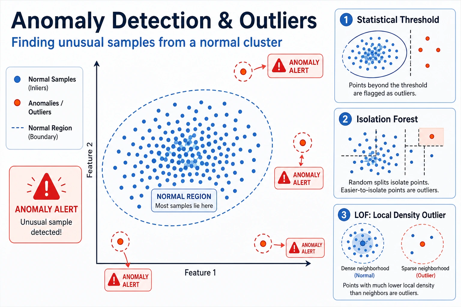
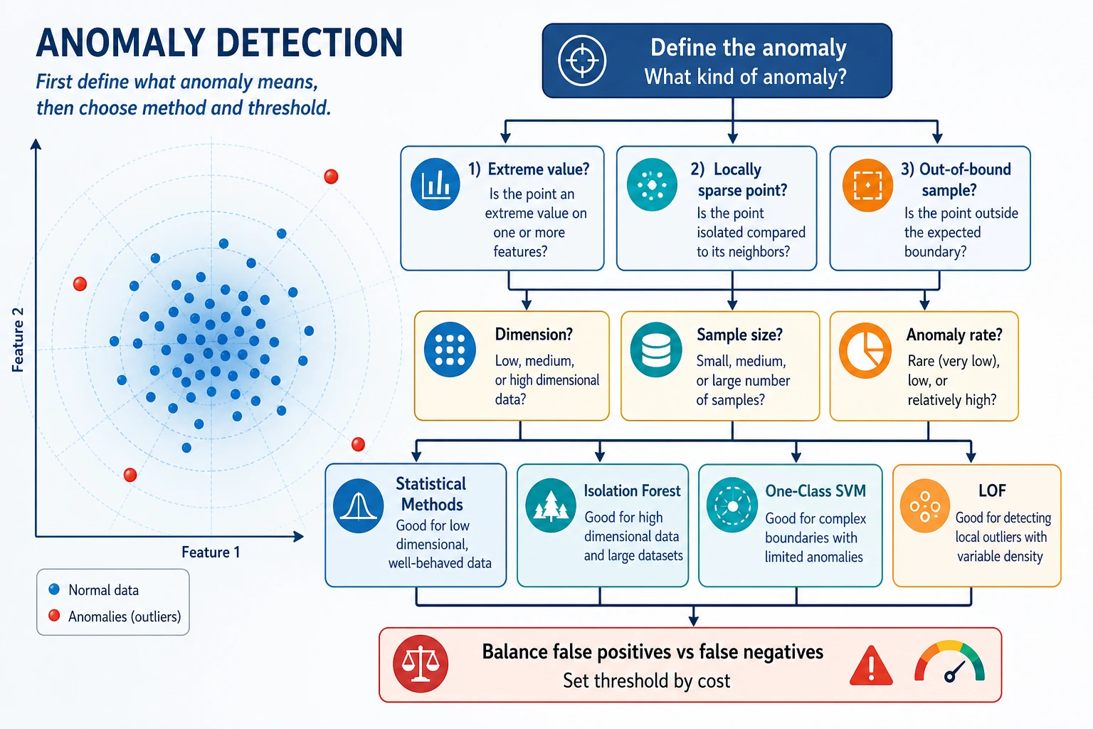
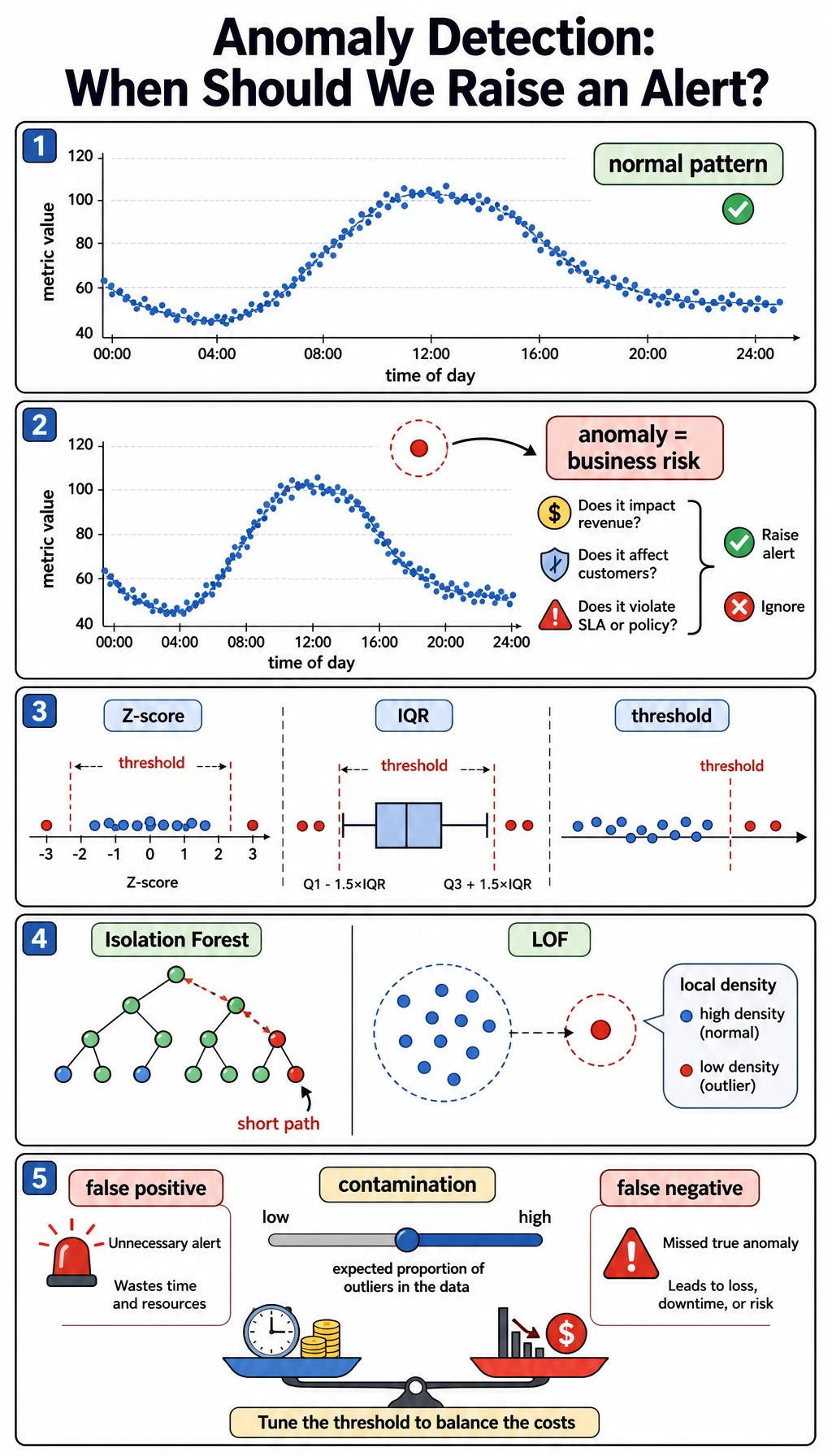
Start with the maps. Anomaly detection is mostly about deciding what to flag and how costly each mistake is.

Keyword Decoder

Term	Practical meaning
anomaly	A sample that does not fit the normal pattern
outlier	A point far from most other points
contamination	Expected fraction of anomalies; used as a threshold hint
score_samples	Model score; for Isolation Forest, lower means more abnormal
false positive	Normal sample incorrectly flagged as suspicious
false negative	Real anomaly missed by the system
IsolationForest	Tree-based method that isolates unusual points quickly
LOF	Local Outlier Factor, compares local density around each point

Setup

python -m pip install -U scikit-learn numpy

This lab uses synthetic labels only to make the lesson measurable. In real anomaly detection, labels are often missing, delayed, or incomplete.

Run the Complete Lab

Create anomaly_lab.py:

import numpy as np
from sklearn.datasets import make_blobs
from sklearn.ensemble import IsolationForest
from sklearn.metrics import confusion_matrix, f1_score, precision_score, recall_score
from sklearn.neighbors import LocalOutlierFactor
from sklearn.preprocessing import StandardScaler


normal, _ = make_blobs(n_samples=360, centers=2, cluster_std=0.75, random_state=42)
rng = np.random.default_rng(42)
outliers = rng.uniform(low=-8, high=8, size=(24, 2))
X = np.vstack([normal, outliers])
y_true = np.array([0] * len(normal) + [1] * len(outliers))  # 1 means anomaly
X_scaled = StandardScaler().fit_transform(X)

print("isolation_forest_contamination_lab")
for contamination in [0.03, 0.06, 0.12]:
    model = IsolationForest(contamination=contamination, random_state=42)
    pred = model.fit_predict(X_scaled)
    y_pred = (pred == -1).astype(int)
    tn, fp, fn, tp = confusion_matrix(y_true, y_pred).ravel()
    print(
        f"contamination={contamination:.2f} "
        f"flagged={int(y_pred.sum())} "
        f"precision={precision_score(y_true, y_pred):.3f} "
        f"recall={recall_score(y_true, y_pred):.3f} "
        f"f1={f1_score(y_true, y_pred):.3f} "
        f"fp={fp} fn={fn}"
    )

print("score_inspection")
best = IsolationForest(contamination=0.06, random_state=42)
best.fit(X_scaled)
scores = best.score_samples(X_scaled)  # lower means more abnormal
order = np.argsort(scores)[:5]
for idx in order:
    print(f"index={idx:<3} score={scores[idx]:.3f} true_anomaly={bool(y_true[idx])}")

print("lof_comparison")
lof = LocalOutlierFactor(n_neighbors=20, contamination=0.06)
y_pred = (lof.fit_predict(X_scaled) == -1).astype(int)
print(
    f"flagged={int(y_pred.sum())} "
    f"precision={precision_score(y_true, y_pred):.3f} "
    f"recall={recall_score(y_true, y_pred):.3f} "
    f"f1={f1_score(y_true, y_pred):.3f}"
)

Run it:

python anomaly_lab.py

Expected output:

isolation_forest_contamination_lab
contamination=0.03 flagged=12 precision=1.000 recall=0.500 f1=0.667 fp=0 fn=12
contamination=0.06 flagged=23 precision=0.826 recall=0.792 f1=0.809 fp=4 fn=5
contamination=0.12 flagged=46 precision=0.478 recall=0.917 f1=0.629 fp=24 fn=2
score_inspection
index=371 score=-0.747 true_anomaly=True
index=368 score=-0.738 true_anomaly=True
index=373 score=-0.734 true_anomaly=True
index=364 score=-0.725 true_anomaly=True
index=378 score=-0.717 true_anomaly=True
lof_comparison
flagged=23 precision=0.870 recall=0.833 f1=0.851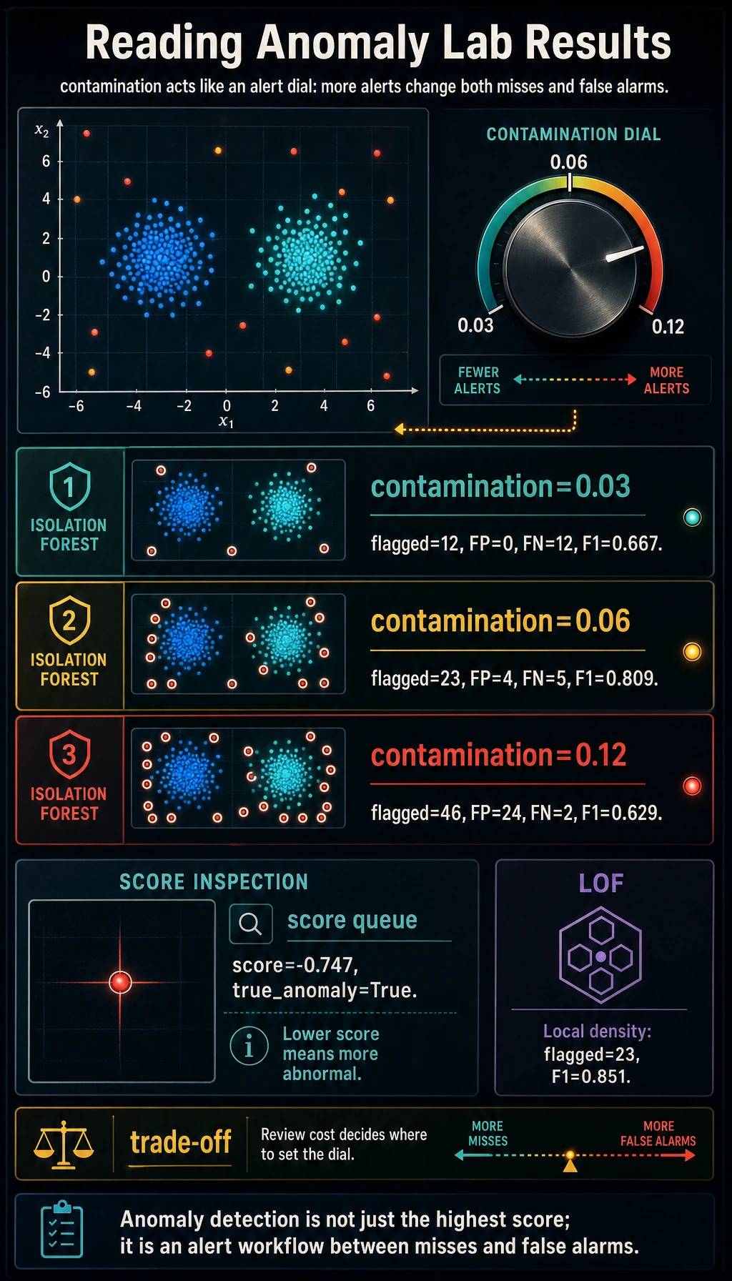

Read the Alert Trade-Off

The contamination value controls how many samples the model expects to flag:

contamination=0.03 flagged=12 precision=1.000 recall=0.500
contamination=0.12 flagged=46 precision=0.478 recall=0.917

This is the same trade-off you saw in classification thresholds:

• lower contamination: fewer alerts, fewer false positives, more missed anomalies;
• higher contamination: more alerts, better recall, more false positives.

The right choice is not purely mathematical. If a missed fraud case is expensive, you may accept more false positives. If manual review is expensive, you may prefer fewer, higher-confidence alerts.

Isolation Forest

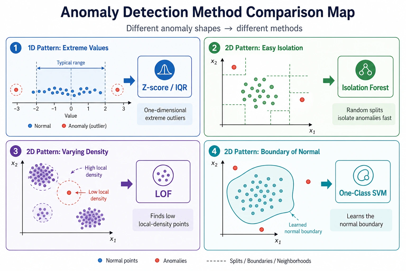
Isolation Forest builds random split trees. Unusual points are often isolated in fewer splits, so they receive more abnormal scores.

In the lab:

scores = best.score_samples(X_scaled)

For Isolation Forest, lower scores are more abnormal. The top suspicious samples were true synthetic anomalies:

index=371 score=-0.747 true_anomaly=True

Use scores when you want to build a review queue instead of only a yes/no prediction.

LOF: Local Density

LOF compares the density around a point with the density around its neighbors. It is useful when an anomaly is not globally far away, but locally strange.

In this synthetic lab:

lof_comparison
flagged=23 precision=0.870 recall=0.833 f1=0.851

LOF performed slightly better than Isolation Forest here. That does not make it universally better. It means the local-density assumption fit this dataset well.

How to Choose a Method

Situation	Good first choice	Why
General tabular anomaly baseline	Isolation Forest	fast, robust, easy to tune
Local density anomalies	LOF	detects points strange relative to neighbors
Simple numeric one-column checks	Z-score or IQR	transparent and cheap
High-dimensional embeddings	Isolation Forest plus neighbor checks	combine score and nearest-neighbor inspection
Need alert operations	Any model plus threshold/review workflow	operations matter as much as score

For experienced readers: anomaly detection should be evaluated with delayed labels, review capacity, alert fatigue, and drift monitoring. A model that maximizes F1 offline may still overload the review team.

Practical Debugging Checklist

Symptom	Likely cause	Fix
Too many alerts	contamination or threshold too high	lower contamination, add review tiers
Many missed anomalies	threshold too strict	increase contamination, add weak rules, monitor recall
Scores change after new data arrives	data distribution drift	monitor score distribution over time
Model flags obvious scale artifacts	features not scaled	scale numeric features first
No labels to evaluate	common in real anomaly work	create a review sample, collect feedback, track delayed outcomes

Practice

1. Change the number of synthetic outliers from 24 to 12 and 48. How should contamination change?
2. Move outliers closer to normal clusters by changing low=-5, high=5. Which method suffers more?
3. Add a fourth feature with a much larger scale. What happens before and after scaling?
4. Sort all samples by score_samples() and inspect the top 20 instead of using a fixed threshold.
5. Design an alert queue with three levels: review now, review later, ignore.

Reference implementation and walkthrough

1. contamination should roughly match the expected anomaly rate, such as 12 / total_samples or 48 / total_samples. In real projects, treat it as an operating assumption and validate it with review results.
2. Moving outliers closer makes every method harder to use. Methods that rely heavily on local density or boundary separation may produce more false negatives; compare ranked examples, not only one metric.
3. A large-scale feature can dominate distance-based behavior before scaling. After scaling, anomaly scores should reflect pattern differences rather than raw units.
4. Ranking by score_samples() is often better for operations because analysts can review the most suspicious cases first even when the final threshold is not settled.
5. A practical queue might send the top 1% to “review now,” the next 4% to “review later,” and the rest to “ignore,” but the exact cutoffs should come from review capacity and false-alarm cost.

Evidence to Keep

Keep this page’s proof of learning as a small evidence card:

Task

clustering, dimensionality reduction, or anomaly detection goal

Data View

scaled features, projection, clusters, or anomaly scores

Interpretation

what the groups, axes, or alerts mean in the scenario

Failure Check

arbitrary cluster count, scaling issue, noisy dimension, or false alert

Expected Output

unsupervised result with interpretation and uncertainty note

Pass Check

You are done when you can explain:

• anomaly detection is an alert workflow, not just a model;
• contamination changes the false-positive/false-negative trade-off;
• Isolation Forest isolates unusual points quickly;
• LOF detects local-density anomalies;
• score inspection is often more useful than a single yes/no label.