6.1.3 From Neurons to Multilayer Perceptrons

Section Overview

A neural network starts with a simple idea: compute a weighted score, pass it through a nonlinear activation, then stack many such units into layers.

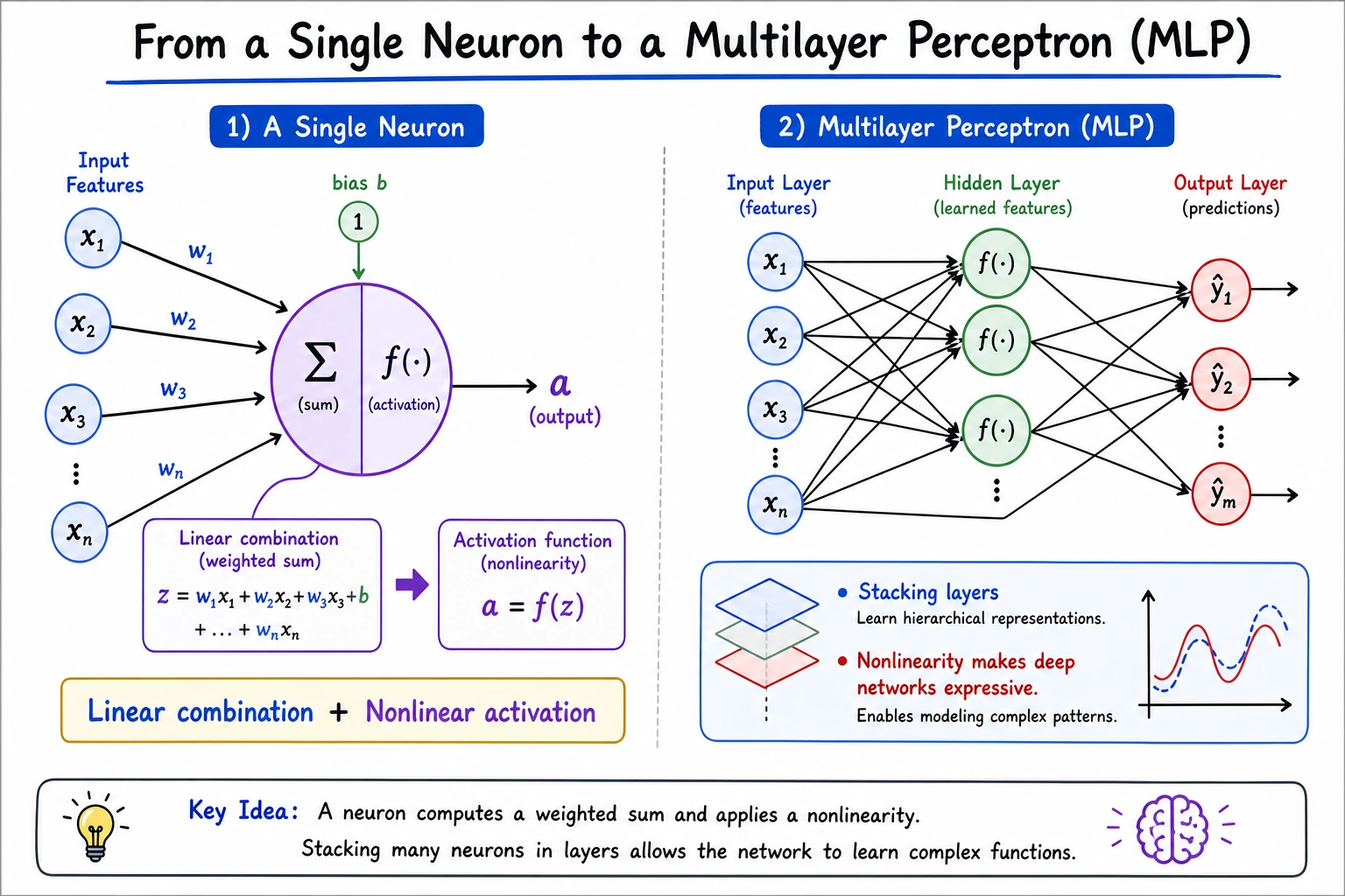
What You Will Build

In this lesson you will run a small PyTorch lab that:

• computes one artificial neuron by hand;
• compares sigmoid and ReLU;
• trains a tiny MLP to solve XOR;
• explains why a single linear layer is not enough.

The key path is:

features→weighted sum z→activation a→layer→multilayer network

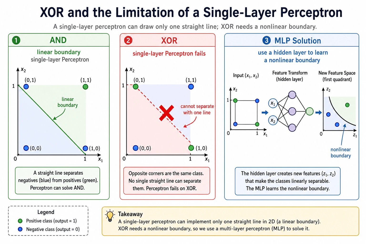
Minimal History

The perceptron was exciting because it showed that a machine could learn a rule from data. It later disappointed people because a single-layer perceptron cannot solve simple nonlinear patterns such as XOR.

That history matters because it gives you the main lesson:

A neuron is simple. Stacking neurons with nonlinear activation is what creates expressive power.

Setup

python -m pip install -U torch

The code uses stable PyTorch APIs: torch.Tensor, nn.Module, nn.Sequential, nn.Linear, activations, loss, and optimizer.

Run the Complete Lab

Create neuron_mlp_lab.py:

import torch
import torch.nn as nn


torch.manual_seed(42)

x = torch.tensor([[0.8, 0.3, 0.5]])
w = torch.tensor([[0.2], [-0.4], [0.6]])
b = torch.tensor([0.1])
z = x @ w + b
print("single_neuron")
print("z=", round(float(z.item()), 3))
print("sigmoid=", round(float(torch.sigmoid(z).item()), 3))
print("relu=", round(float(torch.relu(z).item()), 3))

xor_x = torch.tensor([[0., 0.], [0., 1.], [1., 0.], [1., 1.]])
xor_y = torch.tensor([[0.], [1.], [1.], [0.]])


class TinyMLP(nn.Module):
    def __init__(self):
        super().__init__()
        self.net = nn.Sequential(
            nn.Linear(2, 4),
            nn.Tanh(),
            nn.Linear(4, 1),
            nn.Sigmoid(),
        )

    def forward(self, x):
        return self.net(x)


model = TinyMLP()
loss_fn = nn.BCELoss()
optimizer = torch.optim.Adam(model.parameters(), lr=0.1)

for step in range(2000):
    pred = model(xor_x)
    loss = loss_fn(pred, xor_y)
    optimizer.zero_grad()
    loss.backward()
    optimizer.step()

with torch.no_grad():
    prob = model(xor_x)
    pred = (prob >= 0.5).float()
print("xor_mlp")
for row, p, y_hat in zip(xor_x.tolist(), prob.squeeze().tolist(), pred.squeeze().tolist()):
    print(f"x={row} prob={p:.3f} pred={int(y_hat)}")
print("final_loss=", round(float(loss.item()), 4))

Run it:

python neuron_mlp_lab.py

Expected output:

single_neuron
z= 0.44
sigmoid= 0.608
relu= 0.44
xor_mlp
x=[0.0, 0.0] prob=0.000 pred=0
x=[0.0, 1.0] prob=1.000 pred=1
x=[1.0, 0.0] prob=1.000 pred=1
x=[1.0, 1.0] prob=0.000 pred=0
final_loss= 0.0001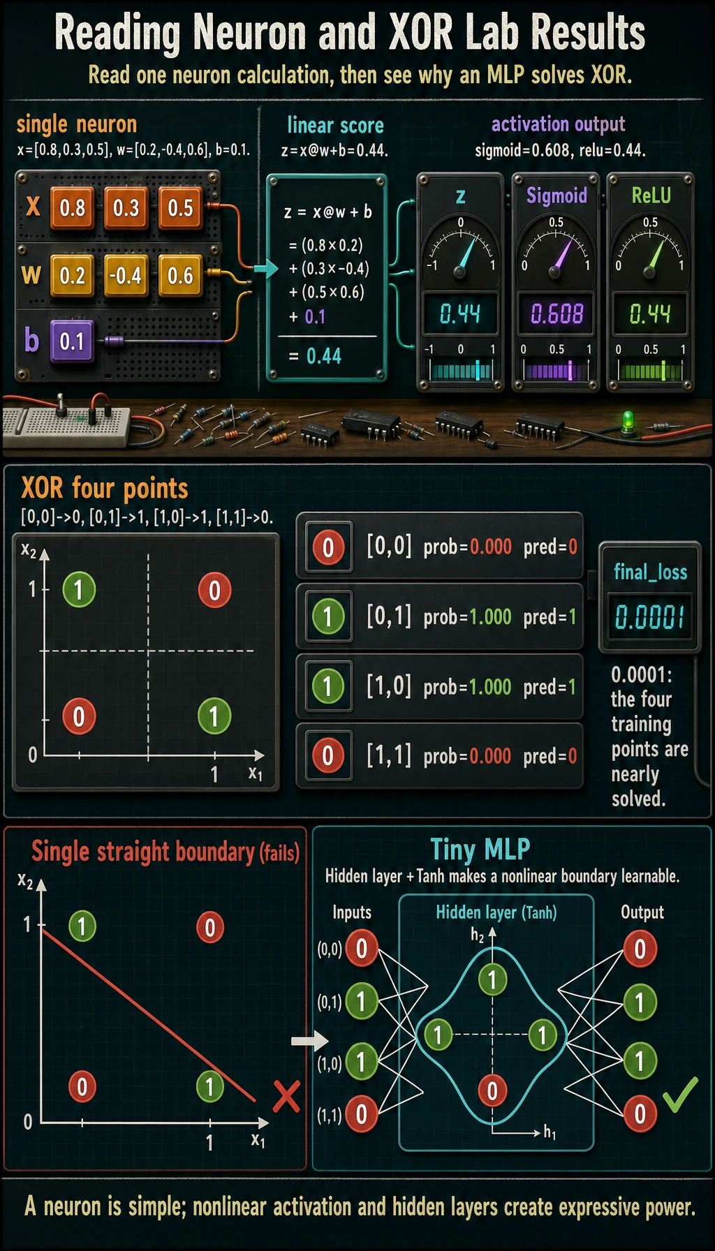

Read One Neuron

The first part computes:

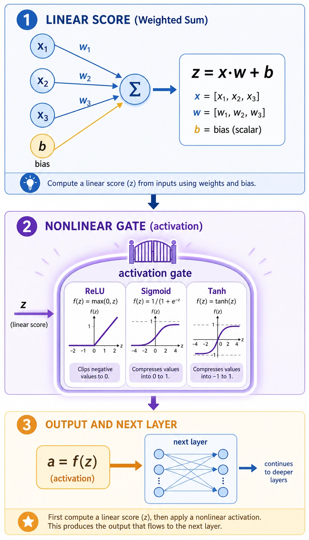
z = x @ w + b

In the output:

z= 0.44
sigmoid= 0.608
relu= 0.44

The weighted score z is still linear. The activation function changes how the signal is passed forward:

Activation	What it does	Common use
Sigmoid	squashes to 0-1	binary probability output
Tanh	squashes to -1 to 1	small demos, some sequence models
ReLU	keeps positive values, zeros negative values	common hidden-layer default

Why Activation Matters

If you stack only linear layers, the whole network is still equivalent to one larger linear layer. Nonlinear activations are what let stacked layers model curved boundaries.

That is why this MLP uses:

nn.Linear(2, 4),
nn.Tanh(),
nn.Linear(4, 1),
nn.Sigmoid(),

The hidden Tanh gives the network nonlinear expressive power. The final Sigmoid turns the output into a probability-like value for binary classification.

Why XOR Is the Classic Test

XOR has only four rows:

x1	x2	y
0	0	0
0	1	1
1	0	1
1	1	0

A straight line cannot separate these labels. That is why a single-layer perceptron fails. A small MLP succeeds because it creates intermediate hidden features before the final decision.

Evidence to Keep

Keep this tiny result card:

Single Neuron

z = x @ w + b, activation changes the signal

Xor Result

[0, 1, 1, 0] recovered by a tiny MLP

Core Reason

nonlinear hidden layers create intermediate features

Failure Probe

remove hidden activation and compare final_loss

The important proof is not that the toy model memorized four rows. The important proof is that nonlinearity changes what a stack of layers can represent.

Practical Debugging Checklist

Symptom	Likely cause	Fix
loss does not decrease	learning rate too high/low, wrong loss	lower LR, check output activation and loss pair
probabilities all near 0.5	model not learning	train longer, inspect gradients, change hidden size
output shape error	target shape differs from prediction	use target shape [batch, 1] for this binary example
values become nan	unstable training	lower learning rate and check inputs
model solves training but not real data	memorization	use train/validation split and regularization

Practice

1. Change hidden units from 4 to 2. Does XOR still train reliably?
2. Replace nn.Tanh() with nn.ReLU(). Does the result change?
3. Print loss every 200 steps to see the training curve.
4. Remove the hidden activation and explain why the model becomes weaker.
5. Add one more hidden layer and compare final loss.

Reference implementation and walkthrough

1. With only 2 hidden units, XOR may still learn, but it becomes less reliable because the network has very little room to build intermediate features.
2. ReLU can work, but the result depends more on initialization and learning rate. Tanh often behaves smoothly on this tiny centered XOR example.
3. A healthy curve should trend downward with small noise. If it stays flat, check learning rate, activation, target shape, and whether optimizer.step() is running.
4. Without a hidden activation, stacked linear layers collapse into one linear transformation. XOR is not linearly separable, so the model loses the key ability it needs.
5. One more hidden layer can help, but it is not automatically better. Compare final loss and stability; if training becomes harder, the extra depth is adding optimization cost.

Pass Check

You are done when you can explain:

• a neuron computes x @ w + b and then applies an activation;
• activation functions add nonlinearity;
• a single-layer perceptron cannot solve XOR;
• an MLP stacks layers to build intermediate features;
• PyTorch models usually combine nn.Module, loss, optimizer, backward(), and step().