3.3.2 Pandas Core Data Structures

Section overview

When many beginners first learn Pandas, they feel that:

• There are too many APIs
• A DataFrame looks like a table, but also like a code object

The most reliable way to understand it is actually:

First think of it as a “labeled table system,” then gradually learn its operations.

In other words, the most important thing in this section is not memorizing every attribute, but first knowing:

• What Series looks like
• What DataFrame looks like
• Why Index keeps showing up

Learning objectives

• Understand the role of Pandas in data analysis
• Master Series creation and basic operations
• Master DataFrame creation and basic attributes
• Understand the Index mechanism

---

First build a map

When learning Pandas for the first time, the safest order is not to “memorize all methods right away,” but to first see clearly:

flowchart LR
    A["Series: a labeled column of data"] --> B["DataFrame: a table made by combining many columns"]
    B --> C["Index: the positioning system for rows and columns"]
    C --> D["All later filtering, cleaning, and aggregation build on these"]

So what this section really wants to solve is:

• Why Pandas is not just “Excel in Python”
• Why Series / DataFrame / Index become the foundation of the whole chapter

---

What is Pandas?

If NumPy is the engine of Python data science, then Pandas is the steering wheel and dashboard—it lets you control and inspect data conveniently.

flowchart LR
    A["Raw data<br/>CSV / Excel / JSON / SQL"] --> B["Pandas<br/>read · clean · analyze"]
    B --> C["Analysis results<br/>statistics · visualization · reports"]

    style B fill:#ff9800,color:#fff,stroke:#e65100

Core capabilities of Pandas:

Capability	Description
Data I/O	Read CSV, Excel, JSON, SQL in one line
Data cleaning	Handle missing values, duplicates, and outliers
Data filtering	Filter and query data flexibly like SQL
Grouped statistics	groupby is dozens of times faster than pure Python loops
Data merging	Merge multiple tables like SQL JOIN

A better beginner-friendly analogy

You can think of Pandas as:

• A smart spreadsheet that remembers row and column labels

A regular list is more like:

• A pile of raw data with no column names

NumPy is more like:

• A matrix engine built for high-speed numerical computing

Pandas is more like:

• The place where you really start working with “fields, row records, and table structures”

Remember the warm-up exercise in Chapter 1? 75 lines of pure Python code did the job, while Pandas did it in just 5 lines. Now let’s formally learn it.

import pandas as pd
import numpy as np

print(pd.__version__)  # e.g. 2.2.0

Import convention

Just like NumPy uses np, Pandas is commonly abbreviated as pd.

---

Series: a one-dimensional array with labels

Series is the most basic Pandas data structure—you can think of it as a NumPy array with labels.

When you first see a Series, what should you focus on?

The most important thing to grasp first is this sentence:

Series = one column of data + one set of labels.

Once this idea is solid, later on when you see:

• Access by label
• Access by position
• Operations on an entire column

it will all feel much smoother.

Creating a Series

import pandas as pd

# Create from a list (auto-generated 0, 1, 2... index)
s1 = pd.Series([85, 92, 78, 95, 88])
print(s1)
# 0    85
# 1    92
# 2    78
# 3    95
# 4    88
# dtype: int64

# Specify the index
s2 = pd.Series(
    [85, 92, 78, 95, 88],
    index=["Chinese", "Math", "English", "Physics", "Chemistry"]
)
print(s2)
# Chinese      85
# Math         92
# English      78
# Physics      95
# Chemistry    88
# dtype: int64

# Create from a dictionary (keys automatically become the index)
scores = {"Chinese": 85, "Math": 92, "English": 78, "Physics": 95}
s3 = pd.Series(scores)
print(s3)

Structure of a Series

Index        Values
──────────   ──────────
Chinese      85
Math         92
English      78
Physics      95
Chemistry    88

Each Series consists of two parts:

• Index: labels used to locate data
• Values: the actual data, with the underlying storage being a NumPy array

A beginner-friendly comparison table to remember first

What you see now	What you can think of it as
Series	A labeled column of data
Index	The “row name” of this column
Values	The actual data itself

This table is great for beginners because it turns abstract terms back into a few more concrete roles.

s = pd.Series([85, 92, 78], index=["Chinese", "Math", "English"])

print(s.index)    # Index(['Chinese', 'Math', 'English'], dtype='object')
print(s.values)   # [85 92 78]  ← This is a NumPy array!
print(s.dtype)    # int64
print(s.shape)    # (3,)
print(len(s))     # 3

Accessing a Series

s = pd.Series([85, 92, 78, 95], index=["Chinese", "Math", "English", "Physics"])

# Access by label
print(s["Math"])      # 92

# Access by position
print(s.iloc[1])      # 92

# Slicing
print(s["Chinese":"English"])  # Label slicing (includes the end!)
# Chinese    85
# Math       92
# English    78

# Boolean indexing
print(s[s >= 90])
# Math       92
# Physics    95

Label slicing vs positional slicing

• Label slicing s["Chinese":"English"]: includes the end
• Positional slicing s.iloc[0:2]: does not include the end (same as Python lists)

This is an easy place for beginners to get confused.

Operations on a Series

s = pd.Series([85, 92, 78, 95], index=["Chinese", "Math", "English", "Physics"])

# Vectorized operations (same idea as NumPy)
print(s + 5)         # Add 5 points to each subject
print(s * 1.1)       # Multiply each subject by 1.1
print(s.mean())      # 87.5  Average score
print(s.max())       # 95    Highest score
print(s.describe())  # Generate descriptive statistics in one line

---

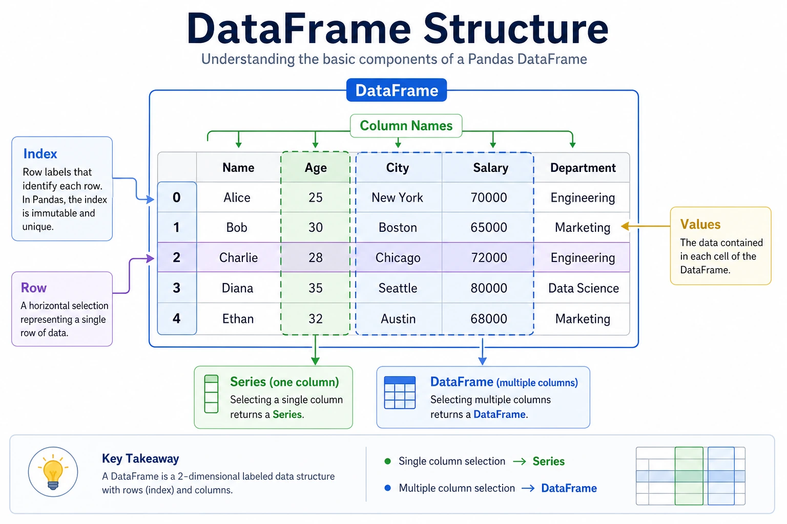
DataFrame: a labeled two-dimensional table

DataFrame is the core of Pandas—you can think of it as an Excel table, or as a dictionary of multiple Series.

When you first see a DataFrame, what should you remember first?

The most important thing to remember is:

DataFrame = multiple Series combined into one table using the same row index.

You can first think of it as:

• A real data table with column names and row numbers

rather than a bunch of arrays stuck together.

Creating a DataFrame

# Method 1: Create from a dictionary (most common)
data = {
    "Name": ["Zhang San", "Li Si", "Wang Wu", "Zhao Liu", "Qian Qi"],
    "Age": [22, 25, 23, 28, 21],
    "City": ["Beijing", "Shanghai", "Guangzhou", "Shenzhen", "Hangzhou"],
    "Salary": [15000, 22000, 18000, 25000, 16000]
}
df = pd.DataFrame(data)
print(df)
#         Name  Age       City  Salary
# 0  Zhang San   22    Beijing   15000
# 1      Li Si   25   Shanghai   22000
# 2    Wang Wu   23  Guangzhou   18000
# 3   Zhao Liu   28   Shenzhen   25000
# 4    Qian Qi   21   Hangzhou   16000

# Method 2: Create from a list of lists
data = [
    ["Zhang San", 22, "Beijing"],
    ["Li Si", 25, "Shanghai"],
    ["Wang Wu", 23, "Guangzhou"]
]
df = pd.DataFrame(data, columns=["Name", "Age", "City"])

# Method 3: Create from a NumPy array
rng = np.random.default_rng(seed=42)
arr = rng.integers(60, 100, size=(5, 3))
df = pd.DataFrame(arr, columns=["Chinese", "Math", "English"])

# Method 4: Create from a dictionary of Series
df = pd.DataFrame({
    "Math": pd.Series([90, 85, 78], index=["Zhang San", "Li Si", "Wang Wu"]),
    "English": pd.Series([88, 92, 75], index=["Zhang San", "Li Si", "Wang Wu"])
})

Structure of a DataFrame

Part	Example
Index	0, 1, 2, 3, 4
Columns	Name, Age, City, Salary
One row	Zhang San, 22, Beijing, 15000

DataFrame = row index (Index) + column names (Columns) + data (Values)

Basic attributes

data = {
    "Name": ["Zhang San", "Li Si", "Wang Wu", "Zhao Liu", "Qian Qi"],
    "Age": [22, 25, 23, 28, 21],
    "City": ["Beijing", "Shanghai", "Guangzhou", "Shenzhen", "Hangzhou"],
    "Salary": [15000, 22000, 18000, 25000, 16000]
}
df = pd.DataFrame(data)

print(df.shape)      # (5, 4)  → 5 rows, 4 columns
print(df.columns)    # Index(['Name', 'Age', 'City', 'Salary'], dtype='object')
print(df.index)      # RangeIndex(start=0, stop=5, step=1)
print(df.dtypes)
# Name      object    ← string
# Age        int64
# City      object
# Salary     int64
print(df.size)       # 20  → 5 × 4 = 20 elements
print(len(df))       # 5   → number of rows

Quickly inspect data

# First 3 rows
print(df.head(3))

# Last 2 rows
print(df.tail(2))

# Basic information
print(df.info())
# <class 'pandas.core.frame.DataFrame'>
# RangeIndex: 5 entries, 0 to 4
# Data columns (total 4 columns):
#  #   Column  Non-Null Count  Dtype
# ---  ------  --------------  -----
#  0   Name      5 non-null      object
#  1   Age       5 non-null      int64
#  2   City      5 non-null      object
#  3   Salary    5 non-null      int64

# Summary statistics for numeric columns
print(df.describe())
#              Age           Salary
# count   5.000000      5.000000
# mean   23.800000  19200.000000
# std     2.774887   4147.288271
# min    21.000000  15000.000000
# 25%    22.000000  16000.000000
# 50%    23.000000  18000.000000
# 75%    25.000000  22000.000000
# max    28.000000  25000.000000

info() and describe() are your friends

When you get a new dataset, the first thing to do is run df.info() and df.describe()—they can help you understand the overall picture of the data in just a few seconds.

A beginner-friendly sequence for a new table

A safer workflow is usually:

1. Check df.head()
2. Check df.info()
3. Check df.describe()
4. Then start filtering and cleaning

This is much less likely to make you lose your way than jumping straight into complex operations.

Accessing columns

# Access a single column → returns a Series
print(df["Name"])
# 0    Zhang San
# 1        Li Si
# ...

# You can also use dot notation (when the column name has no spaces and does not conflict with methods)
print(df.Age)

# Access multiple columns → returns a DataFrame
print(df[["Name", "Salary"]])
#         Name  Salary
# 0  Zhang San   15000
# 1      Li Si   22000
# ...

Why is “learning to read columns first” so important?

Because most Pandas work later on does three things:

• Select columns
• Modify columns
• Perform statistics and combinations based on columns

So when learning Pandas for the first time, instead of rushing to memorize lots of advanced methods, it’s better to first make sure you understand “How do I find this column, what type is it, and what can I do with it?”

Adding and deleting columns

# Add a new column
df["After-Tax Salary"] = df["Salary"] * 0.85
print(df[["Name", "Salary", "After-Tax Salary"]])

# Add a column based on a condition
df["Salary Level"] = np.where(df["Salary"] >= 20000, "High", "Medium")
print(df[["Name", "Salary", "Salary Level"]])

# Delete a column
df = df.drop(columns=["After-Tax Salary"])  # returns a new DataFrame
# or
# df.drop(columns=["After-Tax Salary"], inplace=True)  # modify in place

---

Why Index matters

Index is the key feature that distinguishes Pandas from NumPy.

Setting the index

df = pd.DataFrame({
    "Name": ["Zhang San", "Li Si", "Wang Wu"],
    "Age": [22, 25, 23],
    "Salary": [15000, 22000, 18000]
})

# Set the "Name" column as the index
df_indexed = df.set_index("Name")
print(df_indexed)
#             Age  Salary
# Name
# Zhang San    22   15000
# Li Si        25   22000
# Wang Wu      23   18000

# Access by index
print(df_indexed.loc["Li Si"])
# Age        25
# Salary    22000

# Reset the index
df_reset = df_indexed.reset_index()
print(df_reset)  # same as before

Index alignment

Pandas operations automatically align by index—this is a very powerful feature:

s1 = pd.Series({"Chinese": 85, "Math": 92, "English": 78})
s2 = pd.Series({"Math": 88, "English": 82, "Physics": 90})

# Automatically align by index when adding
result = s1 + s2
print(result)
# English    160.0
# Math       180.0
# Physics      NaN   ← s1 does not have Physics, so the result is NaN
# Chinese      NaN   ← s2 does not have Chinese, so the result is NaN

---

Series vs DataFrame comparison

Feature	Series	DataFrame
Dimension	1D	2D
Analogy	One column in Excel	An entire Excel table
Creation	pd.Series([1,2,3])	pd.DataFrame({"a":[1,2]})
Accessing a column	—	df["column_name"] returns a Series
Index	One Index	Row index + column index

---

Evidence to Keep

Keep this page’s proof of learning as a small evidence card:

Dataframe State

columns, dtypes, row count, missing values, and sample rows

Operation

read/write, select/filter, clean, transform, groupby, merge, or time-series step

Output

resulting table, saved file, aggregation, join result, or time index view

Failure Check

dtype mismatch, missing data, duplicated keys, chained assignment, or wrong time frequency

Expected Output

before/after table sample with the transformation reason

Summary

  root((Pandas Core Data Structures))
    Series
      Labeled one-dimensional array
      index + values
      Like an enhanced dictionary
    DataFrame
      Labeled two-dimensional table
      index + columns + values
      Like an Excel table
    Index
      Automatic alignment
      set_index / reset_index
      Label-based access
    Common methods
      head / tail
      info / describe
      shape / dtypes / columns

---

Hands-on exercises

Exercise 1: Create a Series

# Create a Series representing daily step counts for one week
# Use "Monday" to "Sunday" as the index
# 1. Print the average step count
# 2. Find the day with the most steps
# 3. Find the days with more than 8000 steps

Exercise 2: Create a DataFrame

# Create a feature progress DataFrame containing:
# Feature, Owner, Planned Hours, Actual Hours, Status columns, at least 5 items
# 1. Add a "Delta Hours" column
# 2. Add an "Over Budget" column
# 3. Add a "Risk" column (Blocked -> High, Review -> Medium, Done -> Low, otherwise Watch)
# 4. Use describe() to view statistics for the numeric columns

Exercise 3: Index operations

# Use the DataFrame from Exercise 2
# 1. Set "Feature" as the index
# 2. Find one feature's full progress record by name
# 3. Reset the index

Reference implementation and walkthrough

• For the weekly step-count Series, use weekday names as the index, then compute the mean, max day with idxmax, and filtered high-step days with a boolean condition.
• For the feature progress DataFrame, add Delta Hours and Over Budget, then create Risk with a function, map, or pd.cut depending on your rule. describe() is useful evidence, but it is not the full analysis.
• Index practice should show both set_index and reset_index. A good answer explains when label lookup with .loc is clearer than positional lookup with .iloc.