10.1.2 Digital Image Fundamentals

Learning Objectives

After completing this section, you will be able to:

• Understand pixel representation and color channels in images
• Tell the difference between how grayscale images and color images are stored
• Understand the difference between RGB and HSV
• Know which common image formats are suitable for different scenarios

---

How this section connects to the CNN main track in Station 6

If you just finished convolutional networks, you can first understand this section as:

• CNNs tell you why neural networks are suitable for image understanding
• This section starts by breaking down the input object itself: the image

So this section is not drifting away from the model storyline. Instead, it is filling in the most important layer of input intuition:

• What an image actually is inside a computer
• Why concepts like channels, color spaces, and image size keep showing up later

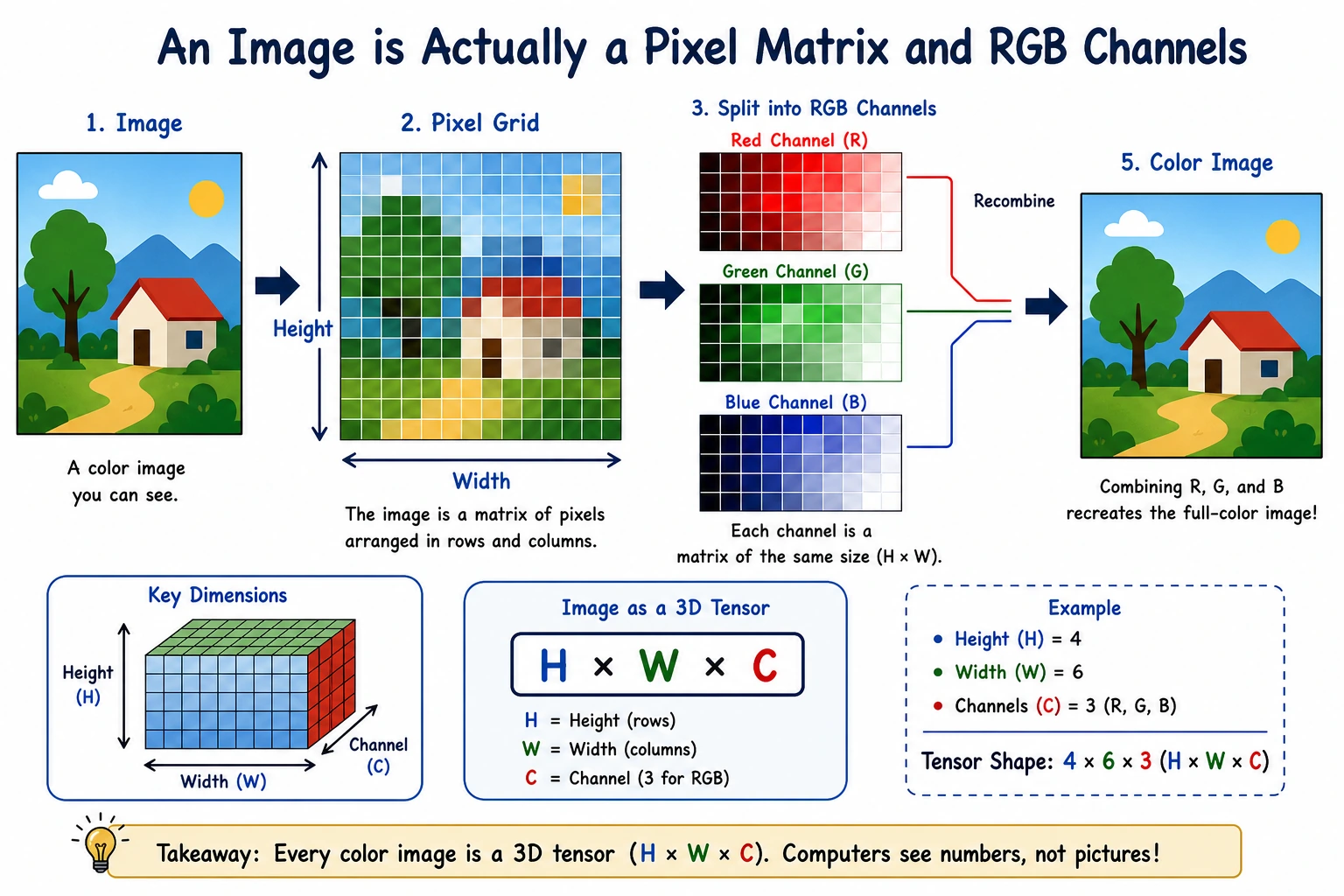
What is a picture in the eyes of a computer?

When people see a photo of a cat, they think, “This is a cat.” What the computer actually sees is not “a cat,” but a bunch of numbers.

The simplest way to think about it is:

Image = a numerical matrix arranged by position

You can think of it as a “grid of lights”:

• Each cell is a pixel
• Each pixel stores a brightness or color value
• All pixels together make up the whole image

What should you focus on first when learning vision for the first time?

What you should focus on first is not “what is in this image,” but:

For a computer, an image is first a spatially arranged numeric grid.

Once this idea is solid, many operations become much easier to understand:

• Why convolutions slide over local windows
• Why channels can be processed separately
• Why detection and segmentation still depend on pixel space

---

Pixels: the smallest unit of an image

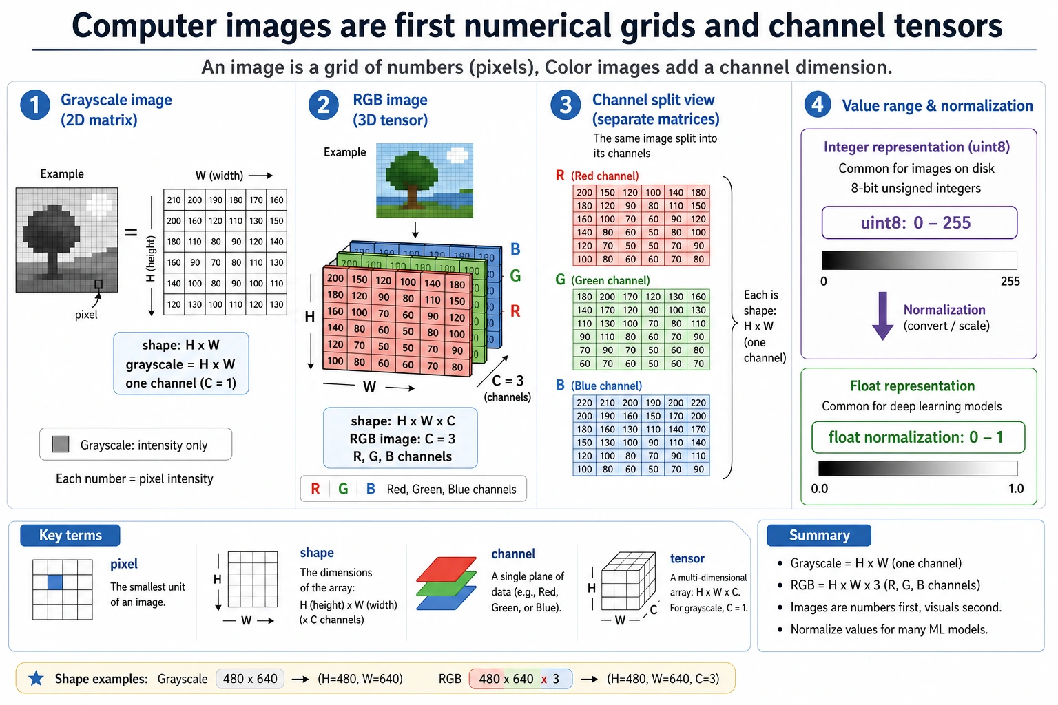
Grayscale images

In a grayscale image, each pixel needs only one number to represent brightness:

• 0 means pure black
• 255 means pure white
• Values in between represent different shades of gray

import numpy as np

# A 5x5 grayscale image
gray = np.array([
    [0,   50, 100, 150, 200],
    [30,  80, 130, 180, 230],
    [60, 110, 160, 210, 255],
    [20,  70, 120, 170, 220],
    [10,  40,  90, 140, 190]
], dtype=np.uint8)

print("Grayscale image shape:", gray.shape)
print(gray)

Expected output:

Grayscale image shape: (5, 5)
[[  0  50 100 150 200]
 [ 30  80 130 180 230]
 [ 60 110 160 210 255]
 [ 20  70 120 170 220]
 [ 10  40  90 140 190]]

Here, shape is (5, 5), which means:

• Height 5
• Width 5

In other words, this image has only 25 pixels.

Color images

Color images are usually represented with RGB:

• R = red intensity
• G = green intensity
• B = blue intensity

Each pixel is no longer a single number, but three numbers.

import numpy as np

# A 2x2 RGB image
rgb = np.array([
    [[255,   0,   0], [  0, 255,   0]],
    [[  0,   0, 255], [255, 255,   0]]
], dtype=np.uint8)

print("RGB image shape:", rgb.shape)
print(rgb)

Expected output:

RGB image shape: (2, 2, 3)
[[[255   0   0]
  [  0 255   0]]

 [[  0   0 255]
  [255 255   0]]]

Here, shape = (2, 2, 3), which means:

• Height 2
• Width 2
• 3 channels per pixel

The most useful habit to build first in this section

When you see an image array, ask these three questions:

1. What is its shape?
2. What does each dimension represent?
3. Are the channels in the last dimension or the first dimension?

This habit will help you avoid a lot of shape confusion in vision code.

Reading tip

Read this figure as height -> width -> channel: grayscale images are usually a 2D grid, RGB images add a color channel, and before training, models also convert uint8 values from 0-255 into a more stable floating-point range.

---

What are channels?

A channel can be understood as a “different color layer” of the same image.

As an analogy:

An RGB image is like three semi-transparent sheets stacked together: one red sheet, one green sheet, and one blue sheet.

import numpy as np

rgb = np.array([
    [[255,   0,   0], [  0, 255,   0]],
    [[  0,   0, 255], [255, 255,   0]]
], dtype=np.uint8)

red_channel = rgb[:, :, 0]
green_channel = rgb[:, :, 1]
blue_channel = rgb[:, :, 2]

print("R channel:\n", red_channel)
print("G channel:\n", green_channel)
print("B channel:\n", blue_channel)

Expected output:

R channel:
 [[255   0]
 [  0 255]]
G channel:
 [[  0 255]
 [  0 255]]
B channel:
 [[  0   0]
 [255   0]]

In computer vision, “splitting channels” is a very common operation.

For example:

• Analyze brightness only
• Enhance a specific color only
• Convert to grayscale first, then do edge detection

What is most important to remember about channels is not the definition, but that they can be processed separately

In other words:

• A color image is not a single black box
• It is actually multiple “color layers” stacked together

This is important because many vision operations later are essentially doing:

• Channel splitting
• Channel recombination
• Separate operations on one channel

---

Why are images often stored as uint8?

Most image pixel values are in the range 0~255, so uint8 is commonly used for storage:

• u = unsigned
• int8 = 8-bit integer
• It can represent 0~255

import numpy as np

pixel = np.array([128, 200, 30], dtype=np.uint8)
print(pixel, pixel.dtype)

Expected output:

[128 200  30] uint8

But during model training, we often normalize images to 0~1:

import numpy as np

pixel = np.array([128, 200, 30], dtype=np.float32)
pixel_normalized = pixel / 255.0

print(pixel_normalized)

Expected output:

[0.5019608  0.78431374 0.11764706]

Why normalize?

Because neural networks prefer data with stable numeric scales. It is like cooking: each seasoning needs a reasonable amount, and you cannot have one measured in “grams” while another is measured in “barrels.”

Why is this directly related to the training main track in Station 6?

Because in Station 6, you already saw that:

• Model training is very sensitive to input scale
• Optimizers and gradients are affected by numeric ranges

So image normalization is not a small trick in vision. It is:

• A standard preparation step before visual data enters the training pipeline

---

What is the difference between RGB and HSV?

RGB: describing colors by “how much red, green, and blue”

RGB is very suitable for storing and displaying images. But it does not match how humans usually describe colors.

For example, people are more likely to say:

• This color is more reddish
• The saturation is high
• Make it a little brighter

At this point, HSV is often more intuitive:

• H = Hue
• S = Saturation
• V = Value

A small example you can run directly

import colorsys

# Red pixel, first map 0~255 to 0~1
r, g, b = 255 / 255, 80 / 255, 80 / 255
h, s, v = colorsys.rgb_to_hsv(r, g, b)

print("HSV:")
print("H =", round(h, 3))
print("S =", round(s, 3))
print("V =", round(v, 3))

Expected output:

HSV:
H = 0.0
S = 0.686
V = 1.0

What are RGB and HSV good for?

Color space	Best suited for
RGB	Storage, display, neural network input
HSV	Color filtering, color segmentation, processing by “hue/brightness”

For example, if you want to “find reddish regions in an image,” HSV is often more convenient than RGB.

---

Convert a color image to grayscale

A grayscale image is not simply the average of the three channels. Usually, it is weighted according to how sensitive the human eye is to different colors.

A common formula is:

gray = 0.299*R + 0.587*G + 0.114*B

import numpy as np

rgb = np.array([
    [[255,   0,   0], [  0, 255,   0]],
    [[  0,   0, 255], [255, 255, 255]]
], dtype=np.float32)

gray = (
    0.299 * rgb[:, :, 0] +
    0.587 * rgb[:, :, 1] +
    0.114 * rgb[:, :, 2]
)

print(gray.astype(np.uint8))

Expected output:

[[ 76 149]
 [ 29 255]]

---

How should you choose an image format?

This is very practical and engineering-oriented knowledge.

Format	Features	Common uses
JPG / JPEG	Lossy compression, small file size	Photos, web display
PNG	Lossless compression, supports transparency	Icons, screenshots, UI assets
WebP	High compression efficiency	Modern web images
BMP	Basically uncompressed, large file size	Teaching, low-level processing

A very practical rule of thumb

• Photos: prefer JPG
• Need a transparent background: prefer PNG
• Want a balance between quality and size: consider WebP

---

Why do vision tasks always mention “resolution”?

Resolution is the size of an image, such as:

• 224 x 224
• 640 x 480
• 1920 x 1080

The higher the resolution:

• The more detail there is
• The more computation is required

It is like looking at a map:

• Zooming in makes it clearer
• But there is also more information to process

That is why many deep learning models first resize images to a fixed size.

---

A small experiment: count image brightness

The following example can help you quickly build the feeling that “an image is just a numeric matrix.”

import numpy as np

gray = np.array([
    [10, 20, 30],
    [100, 120, 140],
    [200, 220, 240]
], dtype=np.uint8)

print("Darkest pixel:", gray.min())
print("Brightest pixel:", gray.max())
print("Average brightness:", gray.mean())

Expected output:

Darkest pixel: 10
Brightest pixel: 240
Average brightness: 120.0

This is very common in vision tasks, for example:

• Checking whether an image is too dark overall
• Performing brightness normalization
• Estimating exposure conditions

---

Evidence to Keep

Keep this page’s proof of learning as a small evidence card:

Input Image

source image or synthetic image used in the run

Array Shape

width, height, channels, dtype, and coordinate convention

Processed Output

grayscale, crop, edge, threshold, or saved intermediate image

Failure Check

channel order, resize distortion, coordinate mistake, or over-processing

Expected Output

before/after image plus the printed shape or pixel values

Common beginner mistakes

Thinking an image is an “object,” not an “array”

To humans, it is an object; to a computer, it starts as an array. Once you accept this, many vision algorithms become much easier to understand.

Confusing image shape

Different libraries may use different conventions:

• NumPy / OpenCV commonly use H x W x C
• PyTorch commonly uses C x H x W

This is something you must be especially careful about when writing models later.

Thinking RGB and HSV are just different names

They are not. They are different ways of representing color, and they are suitable for different processing tasks.

---

Summary

After learning this section, you should build one key intuition:

An image is not mysterious; at its core, it is a numeric matrix with spatial structure.

Whether it is OpenCV processing, convolutional neural networks, or object detection, the essence is always processing these structured numbers.

---

Exercises

1. Create your own 3x3 grayscale image matrix and compute its maximum, minimum, and average values.
2. Create your own 2x2x3 RGB image and print each channel.
3. Manually convert a set of RGB pixels into 0~1 floating-point values to understand the role of normalization.

Solution approach and explanation

1. A good 3x3 grayscale answer prints a (3, 3) array, then uses min(), max(), and mean(). If the matrix is uint8, the pixel values should stay in the 0-255 range, while the mean may print as a floating-point number.
2. For the RGB image, the expected shape is (2, 2, 3). rgb[:, :, 0], rgb[:, :, 1], and rgb[:, :, 2] should each return a 2x2 channel matrix.
3. Normalization means dividing each channel value by 255.0. The relative color does not change, but the numeric range becomes 0-1, which is usually easier for models and later processing.