6.4.2 RNN Basics

Section Overview

CNNs scan space. RNNs scan time. The key idea is simple: read the current step, combine it with a compressed memory from the previous step, and update that memory.

Learning Objectives

• Explain why order matters in sequence tasks.
• Compute a tiny hidden state update by hand.
• Read nn.RNN input/output shapes in PyTorch.
• Build a small many-to-one sequence classifier.
• Understand why plain RNNs struggle with long dependencies.

---

Look at the Hidden-State Loop First

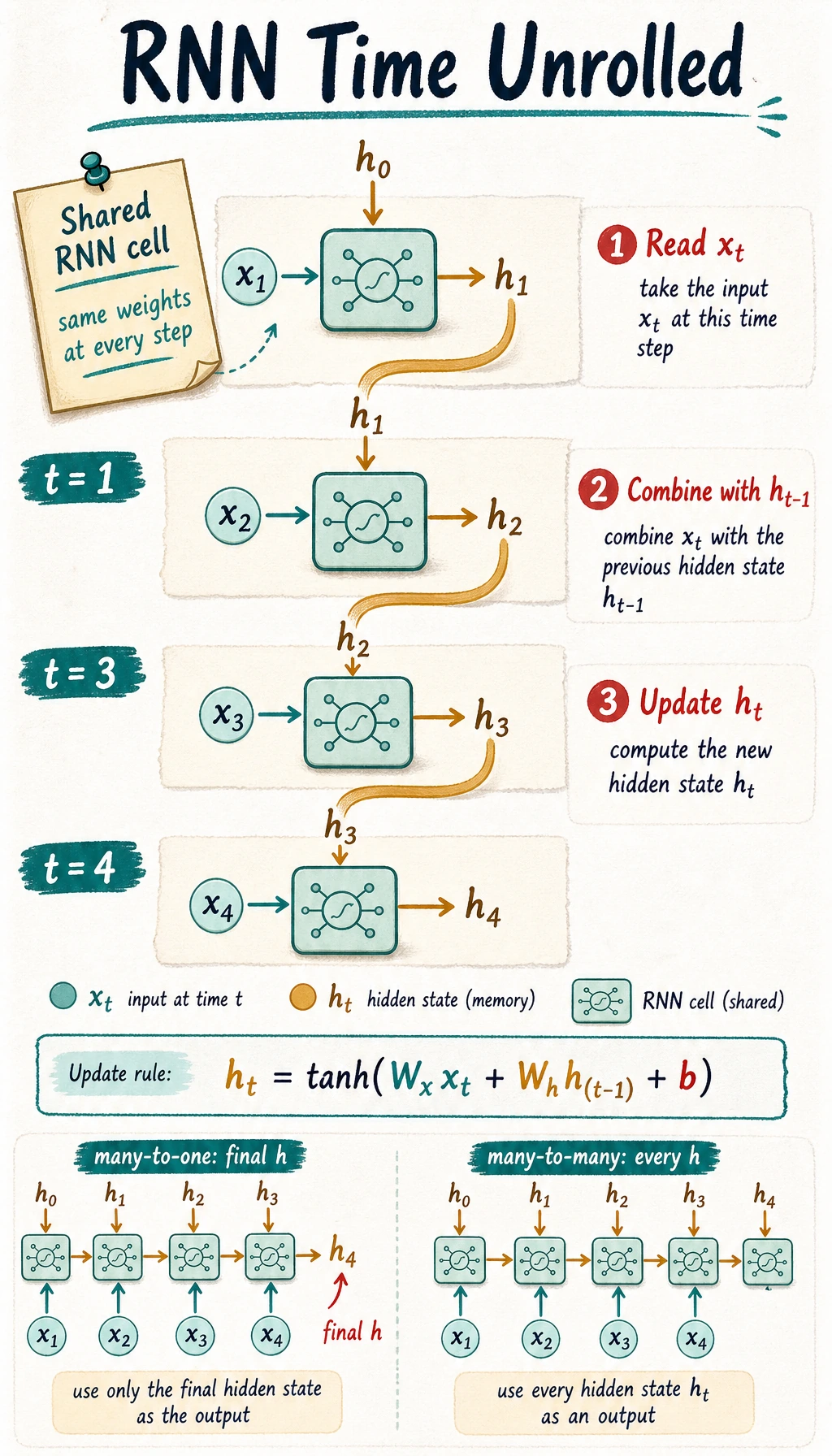
Read the picture like this:

x_t + h_{t-1}→RNN cell→h_t

The same RNN cell is reused at every time step. That is why an RNN can process a sequence of length 5 or 50 without creating a new set of parameters for every position.

Why Sequence Tasks Are Different

Order itself carries information.

Data	Why order matters
sentence	“not good” and “good, not hard” mean different things
stock/sensor series	trend depends on earlier values
user clicks	later actions depend on earlier intent
logs	the same event can mean different things after a previous error

An MLP can process a fixed vector, but it does not naturally carry memory from one step to the next. An RNN adds that missing state.

Lab 1: Manually Update Hidden State

A minimal RNN update can be written as:

h_t = tanh(W_x * x_t + W_h * h_{t-1} + b)

Run a scalar version first:

import numpy as np

x_seq = [1.0, 0.5, -1.0, 2.0]
W_x = 0.8
W_h = 0.5
b = 0.1
h = 0.0

print("manual_rnn_lab")
for t, x_t in enumerate(x_seq, start=1):
    prev_h = h
    h = np.tanh(W_x * x_t + W_h * h + b)
    print(f"step={t} x={x_t:4.1f} prev_h={prev_h: .4f} h={h: .4f}")

Expected output:

manual_rnn_lab
step=1 x= 1.0 prev_h= 0.0000 h= 0.7163
step=2 x= 0.5 prev_h= 0.7163 h= 0.6953
step=3 x=-1.0 prev_h= 0.6953 h=-0.3385
step=4 x= 2.0 prev_h=-0.3385 h= 0.9106

Focus on the dependency:

new h depends on current x and previous h

This is the heart of an RNN.

Lab 2: Read PyTorch RNN Shapes

Use batch_first=True so the input shape is easier to read:

[batch, seq_len, input_size]

Run:

import torch

torch.manual_seed(42)

x = torch.randn(2, 5, 4)
rnn = torch.nn.RNN(input_size=4, hidden_size=6, batch_first=True)
out, h = rnn(x)

print("shape_lab")
print("x:", tuple(x.shape))
print("out:", tuple(out.shape))
print("h:", tuple(h.shape))
print("last_equal:", torch.allclose(out[:, -1, :], h[-1]))

Expected output:

shape_lab
x: (2, 5, 4)
out: (2, 5, 6)
h: (1, 2, 6)
last_equal: True

Read it carefully:

Tensor	Shape	Meaning
x	[2, 5, 4]	2 sequences, 5 steps, 4 features per step
out	[2, 5, 6]	hidden output for every step
h	[1, 2, 6]	final hidden state for 1 layer, batch 2, hidden size 6

For a one-layer RNN, out[:, -1, :] equals h[-1].

Output Patterns

Pattern	Use case	Which output to use
many-to-one	sentiment, trend class, spam class	final hidden state
many-to-many	tagging each token or step	out at every time step
sequence-to-sequence	translation, summarization	encoder/decoder structure

This page focuses on many-to-one because it is the easiest first RNN task.

Lab 3: Train a Tiny Sequence Classifier

The task: classify whether a short numeric sequence is mostly positive or mostly negative.

import torch
from torch import nn

torch.manual_seed(42)

X = torch.tensor(
    [
        [[1.0], [1.2], [1.3], [1.1], [1.0]],
        [[-1.0], [-1.1], [-1.3], [-0.9], [-1.2]],
        [[0.8], [0.7], [1.0], [0.9], [1.1]],
        [[-0.6], [-0.7], [-0.9], [-1.0], [-0.8]],
    ]
)
y = torch.tensor([1, 0, 1, 0])


class SimpleRNNClassifier(nn.Module):
    def __init__(self):
        super().__init__()
        self.rnn = nn.RNN(input_size=1, hidden_size=8, batch_first=True)
        self.fc = nn.Linear(8, 2)

    def forward(self, x):
        out, h = self.rnn(x)
        return self.fc(out[:, -1, :])


model = SimpleRNNClassifier()
loss_fn = nn.CrossEntropyLoss()
optimizer = torch.optim.Adam(model.parameters(), lr=0.05)

for epoch in range(1, 101):
    logits = model(X)
    loss = loss_fn(logits, y)

    optimizer.zero_grad()
    loss.backward()
    optimizer.step()

    if epoch == 1 or epoch % 25 == 0:
        acc = (logits.argmax(1) == y).float().mean().item()
        print(f"trend epoch={epoch:03d} loss={loss.item():.4f} acc={acc:.3f}")

with torch.no_grad():
    result = model(X).argmax(dim=1)

print("predictions:", result.tolist())
print("truth:", y.tolist())

Expected output:

trend epoch=001 loss=0.7726 acc=0.000
trend epoch=025 loss=0.0002 acc=1.000
trend epoch=050 loss=0.0001 acc=1.000
trend epoch=075 loss=0.0000 acc=1.000
trend epoch=100 loss=0.0000 acc=1.000
predictions: [1, 0, 1, 0]
truth: [1, 0, 1, 0]

This is small, but it is a complete RNN loop: sequence tensor, recurrent layer, final hidden representation, classifier, loss, optimizer, and predictions.

Evidence to Keep

Save one RNN run note:

Sequence Shape

[batch, seq_len, input_size]

Rnn Output Shape

[batch, seq_len, hidden_size]

Final State Used

out[:, -1, :] or hidden

Task Result

predictions match truth on the toy task

Limitation

plain hidden state is compressed memory, not perfect memory

Where Plain RNNs Struggle

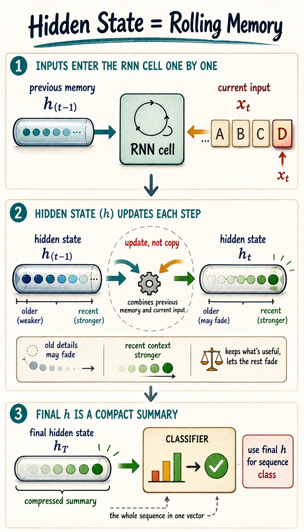
Hidden state is compressed memory, not exact memory. As sequences get long, two problems appear:

Problem	What it means
information washout	early information becomes hard to preserve
vanishing gradients	training signal becomes weak for early steps

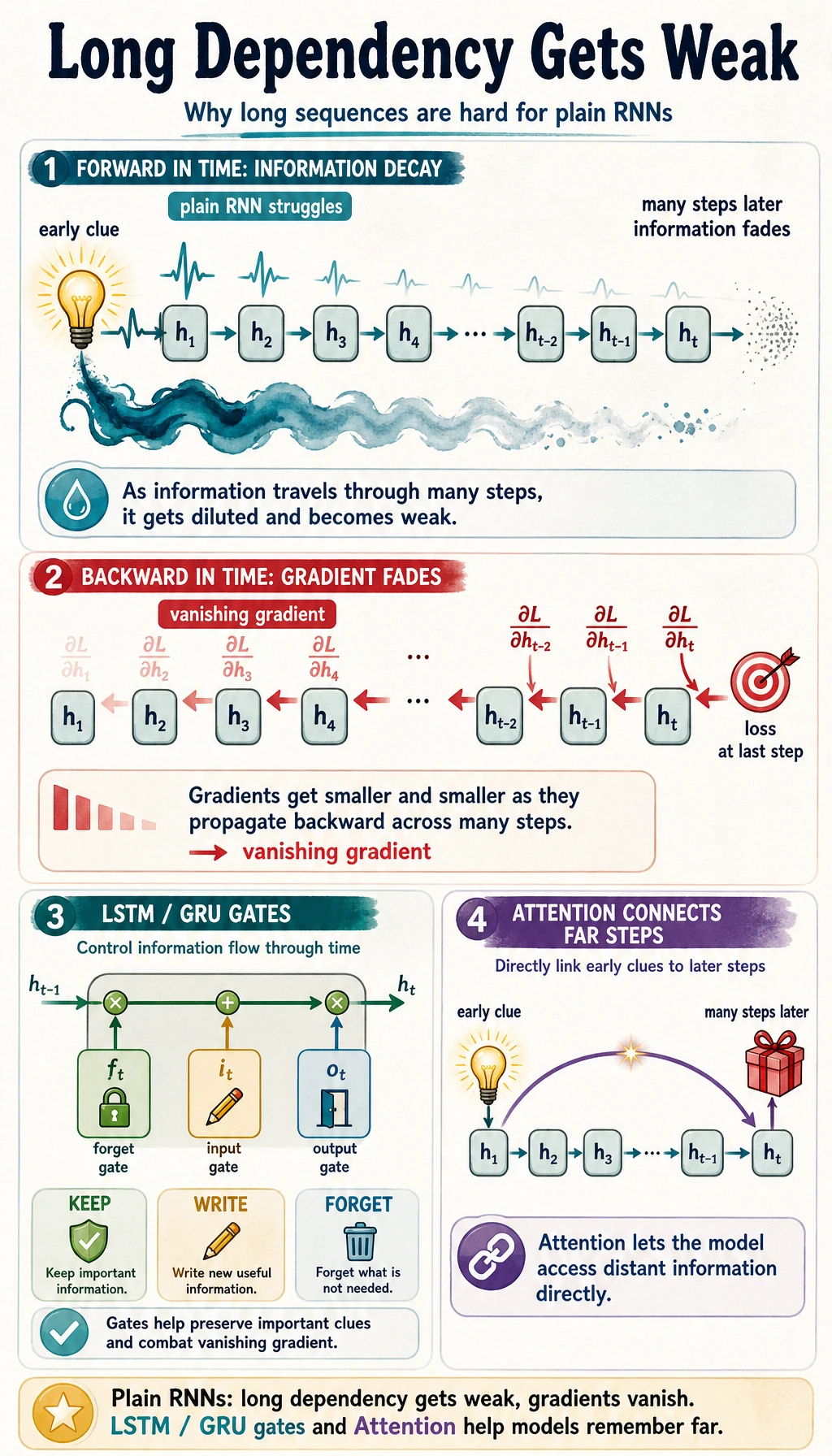
This is why LSTM and GRU add gates: they give the model a better way to keep, update, or discard information.

Common Mistakes

Mistake	Fix
mixing up shape order	with batch_first=True, use [batch, seq_len, input_size]
confusing out and h	out has every step; h is final hidden state per layer
using softmax before CrossEntropyLoss	pass raw logits to the loss
expecting plain RNN to remember everything	use LSTM/GRU or attention for longer dependencies
forgetting sequence length	print tensor shapes before model design

Exercises

1. Change W_h in Lab 1 from 0.5 to 0.9. How does hidden state change?
2. Change hidden_size from 6 to 12 in Lab 2. Which shapes change?
3. In Lab 3, replace the positive/negative sequences with increasing/decreasing sequences.
4. Use out.mean(dim=1) instead of out[:, -1, :] in the classifier. Does it still learn?
5. Explain why a very long sentence is hard for a plain RNN.

Reference implementation and walkthrough

1. A larger W_h makes the previous hidden state carry more strongly into the next step. It may preserve memory better, but it can also amplify instability.
2. Increasing hidden_size changes the last dimension of RNN outputs and hidden states. The classifier input dimension must match the new hidden size.
3. Increasing/decreasing sequences are still order-dependent, so the RNN should learn if the pattern is clear and labels are generated consistently.
4. Mean pooling can work when evidence is spread across the sequence. Last-state pooling is better when the final hidden state is expected to summarize the full history.
5. A plain RNN repeatedly compresses old information into one hidden state. Over long sequences, useful early signals can fade or be overwritten.

Key Takeaways

• RNNs are for ordered data where earlier steps affect later interpretation.
• Hidden state is a compressed rolling memory.
• The same RNN cell is reused across time steps.
• PyTorch RNN input is easiest to read with batch_first=True.
• Plain RNNs are useful for intuition, but LSTM/GRU handle longer dependencies better.