5.3.3 Dimensionality Reduction

Section Overview

Dimensionality reduction compresses many features into fewer features. It can help with visualization, speed, noise reduction, and modeling, but each goal needs a different check.

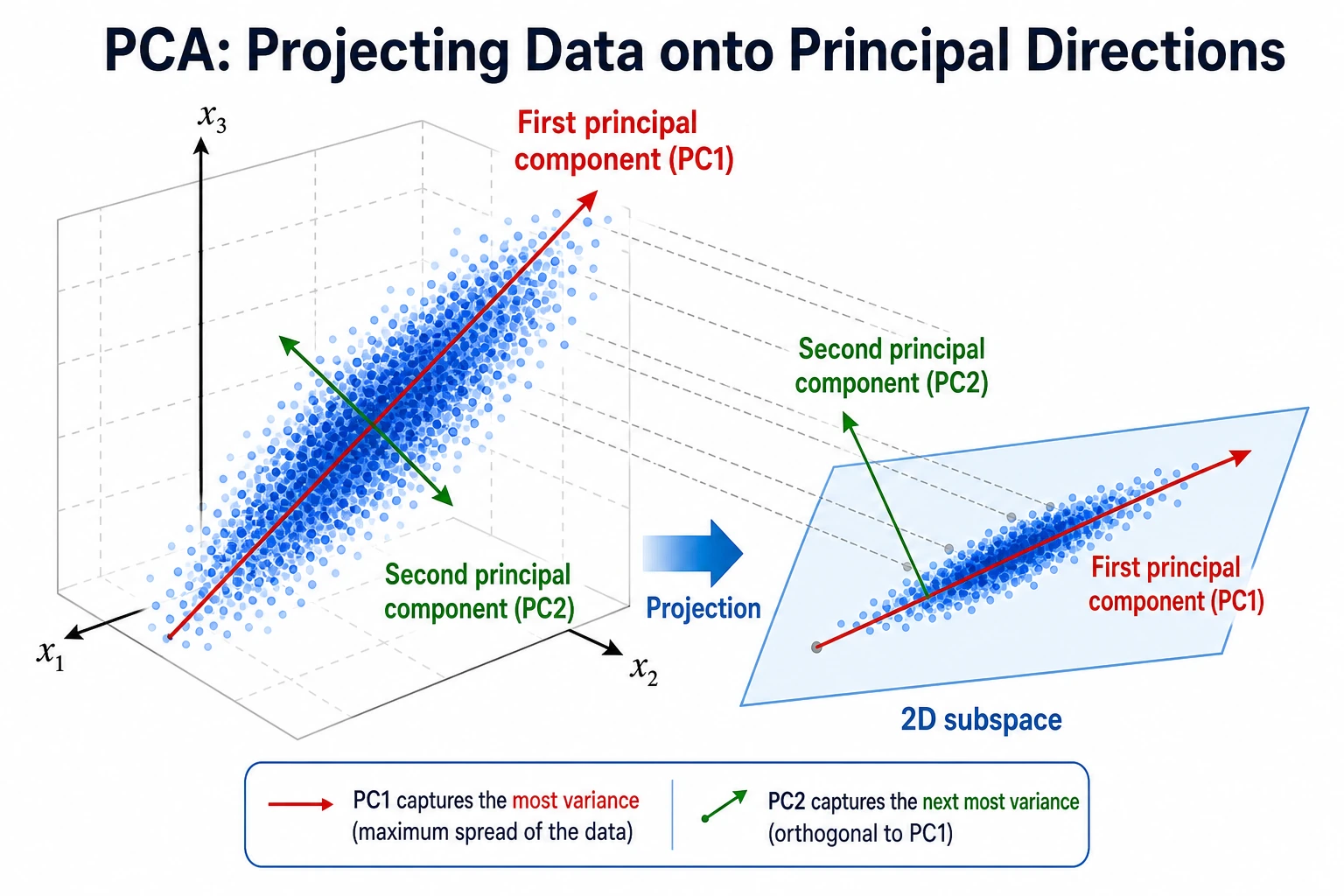
What You Will Build

This lesson uses the handwritten digits dataset to show:

• how PCA maps high-dimensional images into 2 dimensions;
• how explained variance changes when keeping 10, 20, or 40 components;
• how PCA affects classification accuracy;
• how reconstruction error drops as more components are kept;
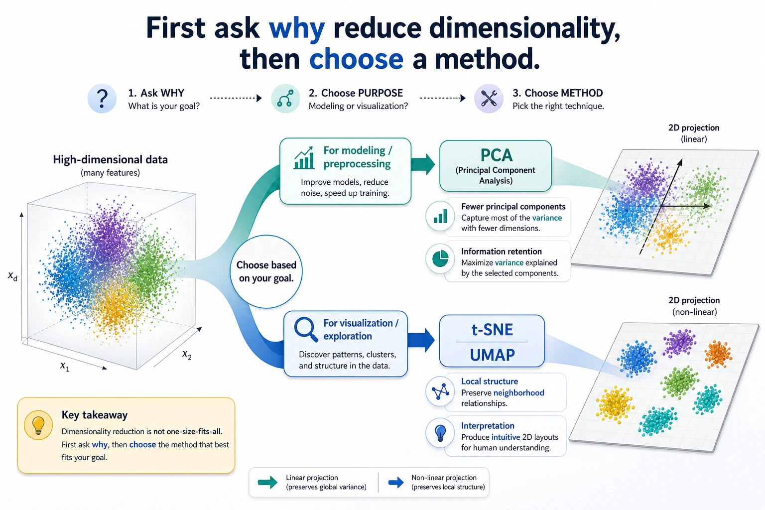
• when PCA, t-SNE, and UMAP should be used differently.

Look at the maps first. Dimensionality reduction is not one tool with one purpose.

Keyword Decoder

Term	Practical meaning
dimension	One feature column, such as one pixel or one numeric field
PCA	Principal Component Analysis; finds directions that keep as much variance as possible
component	A new compressed feature created by PCA
explained_variance_ratio_	How much information-like variance each component keeps
reconstruction	Approximate original data rebuilt from compressed components
t-SNE	Visualization method for local neighborhood structure
UMAP	Visualization and manifold method often used for embeddings

Setup

python -m pip install -U scikit-learn numpy

The runnable lab uses only sklearn and NumPy. UMAP is useful in real projects, but it requires an extra package, so this beginner lab keeps the core dependency small.

Run the Complete Lab

Create pca_lab.py:

import numpy as np
from sklearn.datasets import load_digits
from sklearn.decomposition import PCA
from sklearn.linear_model import LogisticRegression
from sklearn.metrics import accuracy_score, mean_squared_error
from sklearn.model_selection import train_test_split
from sklearn.pipeline import Pipeline
from sklearn.preprocessing import StandardScaler


X, y = load_digits(return_X_y=True)
X_train, X_test, y_train, y_test = train_test_split(
    X, y, test_size=0.25, random_state=42, stratify=y
)

scaler = StandardScaler()
X_train_scaled = scaler.fit_transform(X_train)
X_test_scaled = scaler.transform(X_test)

print("pca_2d_map")
pca2 = PCA(n_components=2, random_state=42)
X_train_2d = pca2.fit_transform(X_train_scaled)
print("shape=", X_train_2d.shape)
print("explained_variance=", np.round(pca2.explained_variance_ratio_, 3).tolist())
print("total_2d_variance=", round(float(pca2.explained_variance_ratio_.sum()), 3))

print("pca_modeling_lab")
for n in [10, 20, 40]:
    model = Pipeline([
        ("scale", StandardScaler()),
        ("pca", PCA(n_components=n, random_state=42)),
        ("clf", LogisticRegression(max_iter=5000, random_state=42)),
    ])
    model.fit(X_train, y_train)
    pred = model.predict(X_test)
    pca = model.named_steps["pca"]
    print(
        f"components={n:<2} "
        f"variance={pca.explained_variance_ratio_.sum():.3f} "
        f"accuracy={accuracy_score(y_test, pred):.3f}"
    )

print("reconstruction_lab")
for n in [10, 20, 40]:
    pca = PCA(n_components=n, random_state=42)
    compressed = pca.fit_transform(X_train_scaled)
    restored = pca.inverse_transform(compressed)
    mse = mean_squared_error(X_train_scaled, restored)
    print(f"components={n:<2} reconstruction_mse={mse:.3f}")

Run it:

python pca_lab.py

Expected output:

pca_2d_map
shape= (1347, 2)
explained_variance= [0.119, 0.097]
total_2d_variance= 0.216
pca_modeling_lab
components=10 variance=0.591 accuracy=0.858
components=20 variance=0.791 accuracy=0.942
components=40 variance=0.953 accuracy=0.960
reconstruction_lab
components=10 reconstruction_mse=0.390
components=20 reconstruction_mse=0.199
components=40 reconstruction_mse=0.045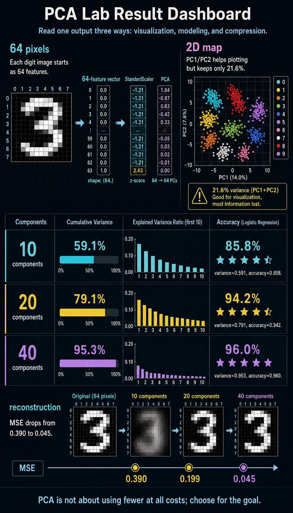

Read the 2D Result

The digits dataset has 64 pixel features. PCA with n_components=2 compresses each image into two numbers:

shape= (1347, 2)
total_2d_variance= 0.216

Two components are useful for plotting, but they keep only about 21.6% of the variance. That is fine for a quick map, but too little for a serious classifier.

Explained Variance

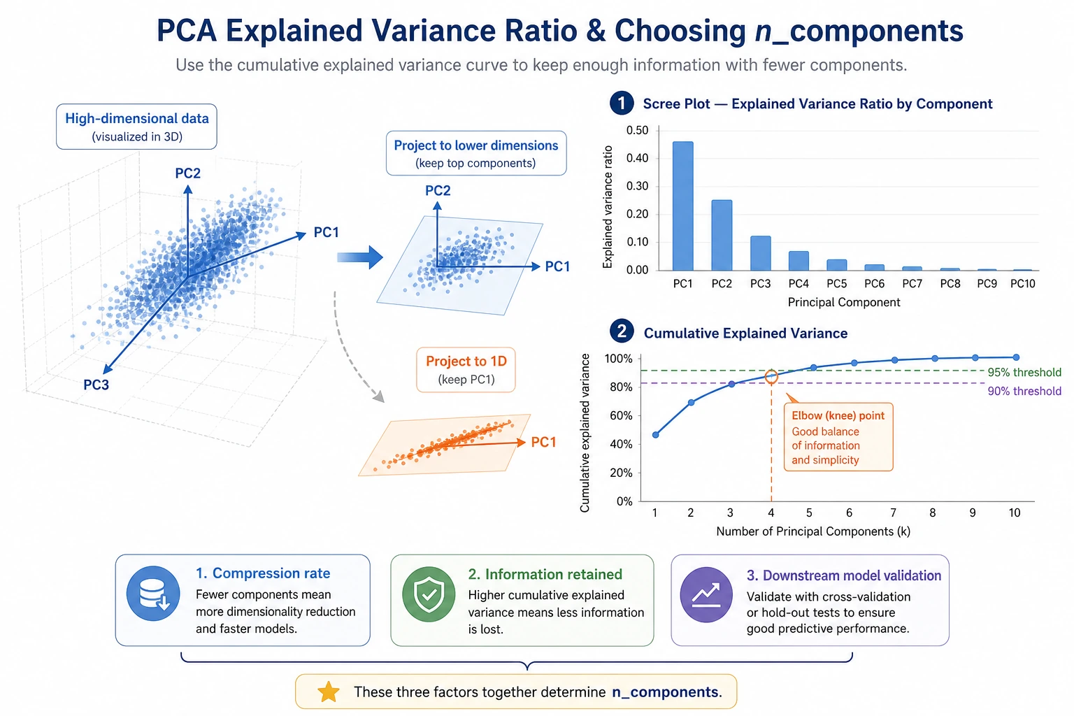
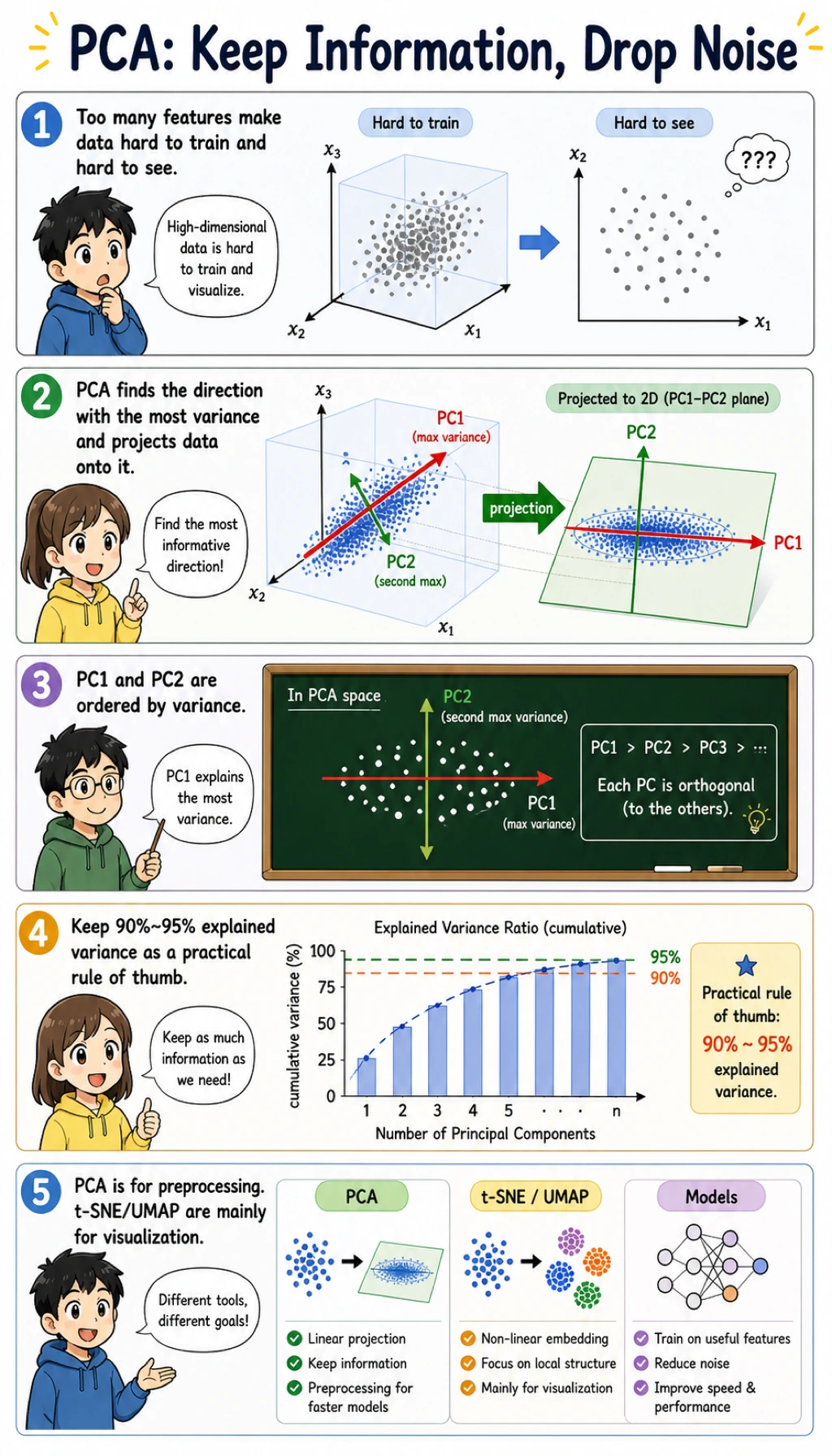
Explained variance helps you decide how much information to keep:

components=10 variance=0.591 accuracy=0.858
components=20 variance=0.791 accuracy=0.942
components=40 variance=0.953 accuracy=0.960

The useful lesson is not “always keep 95%.” The useful lesson is:

• if the goal is visualization, 2 or 3 components may be enough;
• if the goal is modeling, compare accuracy or the metric your project uses;
• if the goal is compression, compare reconstruction error and storage cost.

Reconstruction Error

Reconstruction asks: after compression, how much of the original data can be rebuilt?

components=10 reconstruction_mse=0.390
components=40 reconstruction_mse=0.045

More components make reconstruction better, but they also keep more dimensions. The right number is a trade-off between compactness and useful information.

PCA in a Model Pipeline

The modeling block uses:

Pipeline([
    ("scale", StandardScaler()),
    ("pca", PCA(n_components=n, random_state=42)),
    ("clf", LogisticRegression(max_iter=5000, random_state=42)),
])

This order matters:

1. split train/test first;
2. fit scaling on training data only;
3. fit PCA on training data only;
4. train the model on compressed training features;
5. evaluate on transformed test features.

Putting scaling and PCA in a pipeline helps prevent data leakage during cross-validation.

PCA, t-SNE, and UMAP

Method	Best use	Important warning
PCA	compression, preprocessing, fast 2D overview	linear method; may miss curved structure
t-SNE	local-neighborhood visualization	distances between far clusters can be misleading
UMAP	embedding visualization and neighborhood exploration	needs extra package; tune parameters and verify stability

For beginners, the safest order is:

1. Start with PCA because it is fast and interpretable.
2. Use t-SNE or UMAP for visualization, not as your first production feature pipeline.
3. If dimensionality reduction changes a model, validate with cross-validation.

Practical Debugging Checklist

Symptom	Likely cause	Fix
PCA result dominated by one feature	features are not scaled	use StandardScaler before PCA
2D plot looks nice but model is weak	2D kept too little variance	use more components for modeling
Accuracy drops sharply after PCA	too many useful features were discarded	increase n_components, compare with no-PCA baseline
Cross-validation score is too good	PCA fitted before split	put PCA inside Pipeline
t-SNE/UMAP plot looks overinterpreted	visualization layout is not a proof	check stability and downstream usefulness

Practice

1. Change PCA components to [5, 15, 30, 50]. Where does accuracy stop improving?
2. Run the classifier without PCA. Is PCA helping speed, accuracy, or only compression?
3. Remove StandardScaler. How does explained variance change?
4. Use PCA(n_components=0.95) and print the number of components selected.
5. Use the 2D PCA output to draw a scatter plot colored by digit label.

Operation guide and checkpoints

1. Accuracy often improves quickly at first and then plateaus. The practical answer is the smallest component count whose score is near the best score.
2. PCA may help speed and storage even if accuracy is similar. If accuracy drops, the compressed representation is losing useful signal; if accuracy rises slightly, PCA may be removing noise.
3. Without scaling, features with larger numeric ranges dominate the principal components. Explained variance may look high for the wrong reason.
4. PCA(n_components=0.95) selects the minimum number of components that preserve about 95% of variance. Report both the count and whether the downstream score remains acceptable.
5. A 2D PCA plot is a diagnostic, not proof of model quality. Overlapping colors suggest the classifier needs more dimensions or a nonlinear representation.

Evidence to Keep

Keep this page’s proof of learning as a small evidence card:

Task

clustering, dimensionality reduction, or anomaly detection goal

Data View

scaled features, projection, clusters, or anomaly scores

Interpretation

what the groups, axes, or alerts mean in the scenario

Failure Check

arbitrary cluster count, scaling issue, noisy dimension, or false alert

Expected Output

unsupervised result with interpretation and uncertainty note

Pass Check

You are done when you can explain:

• PCA creates new compressed features called components;
• 2D PCA is useful for visualization but may discard too much information for modeling;
• explained variance is a guide, not an automatic target;
• PCA must be fitted inside the training pipeline;
• t-SNE and UMAP are mainly visualization tools unless you validate them carefully.