6.2.2 From sklearn to PyTorch

Section positioning

If scikit-learn is like an automatic car, then PyTorch is more like a manual car.

• scikit-learn wraps up many details for you
• PyTorch lets you control the model, loss function, gradients, and training process yourself

By learning this section, you’ll know exactly where you are “shifting gears.”

Learning objectives

• Understand the difference in responsibilities between sklearn and PyTorch
• Build a mental model of data, model, loss function, optimizer, and training loop as a whole
• Run a minimal example in both sklearn and PyTorch
• Understand why deep learning needs a more “low-level” framework like PyTorch

---

Why learn PyTorch after learning sklearn?

In Station 5, you already used scikit-learn:

from sklearn.linear_model import LinearRegression

model = LinearRegression()
model.fit(X_train, y_train)
pred = model.predict(X_test)

This experience is very smooth, but it also means many things are being “hidden”:

What you do	What sklearn does for you
Choose a model	Defines the parameter structure
Call fit()	Automatically performs forward computation, computes loss, computes gradients, and updates parameters
Call predict()	Automatically performs inference

In PyTorch, these steps need to be written separately:

Step	What you need to handle yourself
Prepare data	Convert data into Tensor
Define model	Write the network with nn.Module or nn.Sequential
Define loss function	For example, nn.MSELoss()
Define optimizer	For example, torch.optim.SGD()
Training loop	forward -> loss -> backward -> step

This may look more troublesome, but the benefits are:

• You can define any network structure
• You can control every step of the training process
• You can do things that sklearn can hardly cover, such as CNNs, RNNs, Transformers, and fine-tuning large models

---

Looking at both side by side

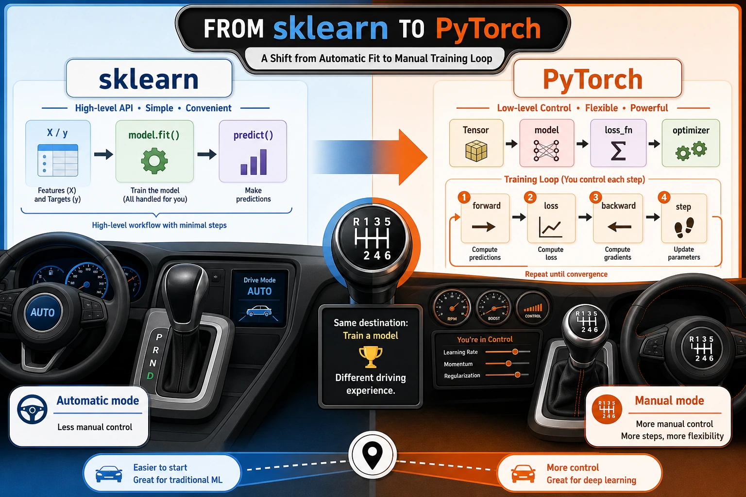
• In sklearn, this whole chain is mostly wrapped inside fit()
• In PyTorch, this chain is fully exposed

So the key thing to learn in PyTorch is not “a few more APIs,” but: you start to truly work with the internal structure of model training.

---

A minimal comparison experiment

Runtime environment

The following code can be run directly. If you have not installed the dependencies locally:

pip install numpy scikit-learn torch

Let’s do the simplest linear regression task: given study time, predict exam score.

Train with sklearn

import numpy as np
from sklearn.linear_model import LinearRegression

# Study time (hours)
X = np.array([[1.0], [2.0], [3.0], [4.0], [5.0]], dtype=np.float32)

# Corresponding scores
y = np.array([52.0, 59.0, 66.0, 73.0, 80.0], dtype=np.float32)

sk_model = LinearRegression()
sk_model.fit(X, y)

print("sklearn intercept:", round(float(sk_model.intercept_), 2))
print("sklearn weight:", round(float(sk_model.coef_[0]), 2))
print("Predicted score for 6 hours of study:", round(float(sk_model.predict([[6.0]])[0]), 2))

Expected output:

sklearn intercept: 45.0
sklearn weight: 7.0
Predicted score for 6 hours of study: 87.0

You get a straight-line model, and the process is very smooth: fit() has already found the line score = 7 * hours + 45.

Train the same task with PyTorch

import torch
from torch import nn

torch.manual_seed(42)

# 1. Convert data to tensors
X_torch = torch.tensor([[1.0], [2.0], [3.0], [4.0], [5.0]])
y_torch = torch.tensor([[52.0], [59.0], [66.0], [73.0], [80.0]])

# 2. Define the model: a linear layer y = wx + b
model = nn.Linear(in_features=1, out_features=1)

# 3. Define the loss function
loss_fn = nn.MSELoss()

# 4. Define the optimizer
optimizer = torch.optim.SGD(model.parameters(), lr=0.01)

# 5. Training loop
for epoch in range(1000):
    pred = model(X_torch)                  # forward
    loss = loss_fn(pred, y_torch)          # compute loss

    optimizer.zero_grad()                  # clear old gradients
    loss.backward()                        # backward
    optimizer.step()                       # update parameters

    if epoch % 200 == 0:
        print(f"epoch={epoch:4d}, loss={loss.item():.4f}")

weight = model.weight.item()
bias = model.bias.item()
pred_6 = model(torch.tensor([[6.0]])).item()

print("PyTorch intercept:", round(bias, 2))
print("PyTorch weight:", round(weight, 2))
print("Predicted score for 6 hours of study:", round(pred_6, 2))

Expected output:

epoch=   0, loss=4031.2007
epoch= 200, loss=72.9774
epoch= 400, loss=18.8304
epoch= 600, loss=4.8588
epoch= 800, loss=1.2537
PyTorch intercept: 43.67
PyTorch weight: 7.37
Predicted score for 6 hours of study: 87.88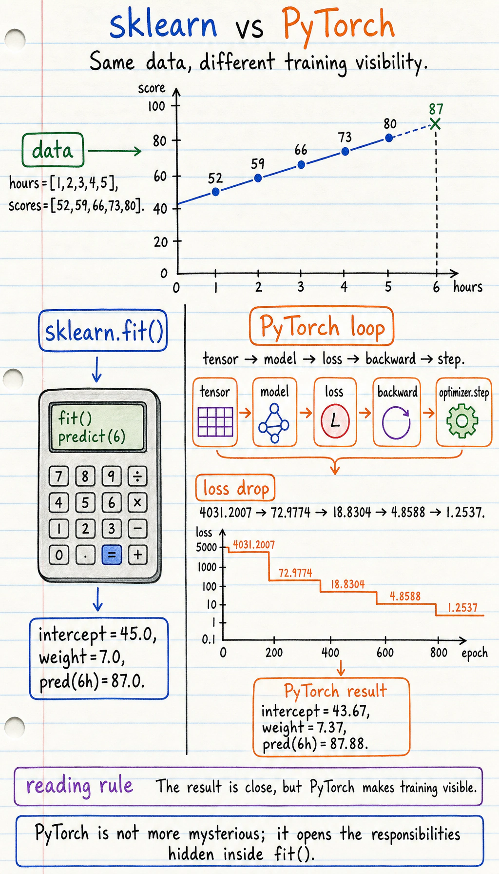

Read the picture from top to bottom:

• sklearn gives an exact line for this tiny dataset, then directly predicts 87.0
• PyTorch starts from random parameters, repeatedly lowers loss, and ends near the same line
• The important difference is not the destination, but how much of the training process you can see and control

---

What did you actually learn here?

Although the PyTorch code is longer than sklearn, it reveals the five core components of deep learning:

Component	Analogy	Role
Data	Ingredients	The input the model processes
Model	Chef	Decides how to turn input into output
Loss function	Score sheet	Judges how well the model performs
Optimizer	Parameter tuner	Changes parameters based on error
Training loop	Daily review	Repeats trial and error until performance improves

Later, when you learn CNNs, Transformers, RAG fine-tuning, or local model training, the essence is still these five things—only the model structure becomes more complex.

---

When should you keep using sklearn, and when should you switch to PyTorch?

Cases better suited to sklearn

• Mainly tabular data
• Models such as linear regression, logistic regression, tree models, random forests, and XGBoost
• You care more about fast modeling and tuning

Cases better suited to PyTorch

• Unstructured data such as images, speech, and text
• Need to customize the network structure
• Need GPU training
• Need to fine-tune pretrained models
• Need to control training details yourself

A simple memory aid:

sklearn is good at the efficient application of “traditional machine learning,” while PyTorch is good at the flexible construction of “deep learning.”

---

Common misconceptions

Misconception 1: PyTorch is just another modeling library

Not quite. It is more like a “deep learning development platform.” You are not just calling models—you are building a training system.

Misconception 2: PyTorch is more advanced than sklearn, so you should use it for everything

That is not true either. In engineering, the most important thing is to choose the right tool. For many tabular tasks, sklearn and tree-based models are still the first choice.

Misconception 3: As long as you can write a training loop, you understand deep learning

The training loop is only the outer shell. You still need to understand:

• Tensors and automatic differentiation
• nn.Module
• Data loading
• Model debugging
• Training stability and evaluation methods

These are the topics that the next sections of this chapter will cover.

---

What you should be able to do after this chapter

After learning this section, you should be able to answer at least these three questions:

1. What steps does sklearn.fit() hide for you?
2. Why can’t PyTorch training avoid the loss function and optimizer?
3. Why do “model + loss + optimizer + training loop” become the common structure of all later deep learning courses?

If you can explain these three questions clearly, then the bridge has been built.

---

Evidence to Keep

Save a side-by-side note:

Sklearn

fit() hides parameter updates

Pytorch

I write model, loss, backward, optimizer step

Same Goal

minimize error and validate on held-out data

New Responsibility

inspect shape, gradient, device, and checkpoint

The point is not that PyTorch is “more advanced.” The point is that PyTorch makes the training mechanism visible enough for custom deep learning systems.

Exercises

1. Change the study time and scores in the example above to your own data, then train once with sklearn and once with PyTorch.
2. Change the learning rate in PyTorch from 0.01 to 0.1 and 0.001, and observe how the loss decreases at different speeds.
3. Try printing weight and bias every 100 epochs to see how the parameters gradually move toward the answer.

Reference implementation and walkthrough

1. The two models should learn a similar line if the data is close to linear. They may not match exactly because sklearn solves the closed-form or optimized regression objective directly, while the PyTorch version moves by gradient steps.
2. 0.1 often learns faster but may overshoot on small or poorly scaled data. 0.001 is usually safer but visibly slower, so the loss curve may still be descending when training stops.
3. weight and bias should move toward values that make predictions closer to the scores. If they stop changing while loss is still high, check the learning rate, tensor shapes, and whether gradients are being applied.