6.2.4 Autograd

Section Overview

autograd is the engine that turns a forward computation into gradients. The important part is not memorizing backward(), but knowing what graph is recorded, where gradients are stored, when they accumulate, and when tracking should be disabled.

Learning Objectives

• Explain what requires_grad=True changes.
• Run loss.backward() and inspect .grad.
• Understand that backward() computes gradients but does not update parameters.
• Avoid gradient accumulation bugs with zero_grad().
• Use torch.no_grad() and detach() in the right places.

---

Look at the Computation Graph First

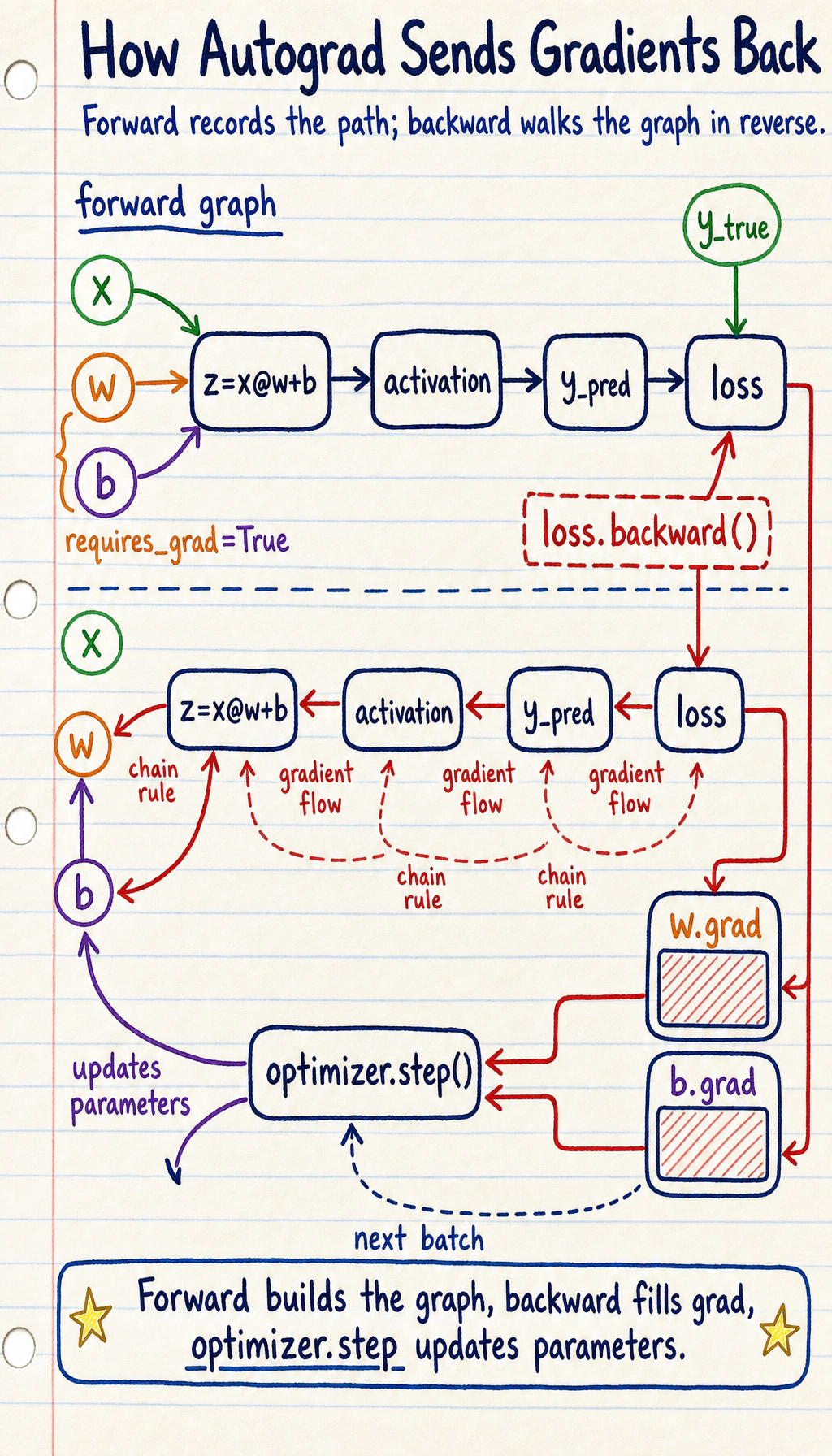
Read the graph like this:

parameter→forward operations→loss→backward()→parameter.grad→optimizer step

Autograd records the operations that produce the loss. When you call backward(), PyTorch walks that recorded graph backward and applies the chain rule.

Lab 1: One Parameter, One Gradient

Start with one number so the mechanism is visible.

import torch

w = torch.tensor(2.0, requires_grad=True)
loss = (w * 3 - 10) ** 2

print("loss:", loss.item())
loss.backward()
print("w.grad:", w.grad.item())

Expected output:

loss: 16.0
w.grad: -24.0

What happened:

• w is a learnable value because requires_grad=True.
• loss is built from w, so PyTorch records the path from w to loss.
• loss.backward() computes how the loss changes if w changes.
• The result is stored in w.grad.

The chain is:

w→w * 3→w * 3 - 10→square→loss

Lab 2: Gradient Is Not the Update

backward() only computes gradients. You still need an update step.

import torch

w = torch.tensor(2.0, requires_grad=True)
lr = 0.1

print("single_parameter_training")
for step in range(1, 6):
    loss = (w * 3 - 10) ** 2
    loss.backward()

    with torch.no_grad():
        w -= lr * w.grad

    print(
        f"step={step} "
        f"w={w.item():.4f} "
        f"loss={loss.item():.4f} "
        f"grad={w.grad.item():.4f}"
    )

    w.grad.zero_()

Expected output:

single_parameter_training
step=1 w=4.4000 loss=16.0000 grad=-24.0000
step=2 w=2.4800 loss=10.2400 grad=19.2000
step=3 w=4.0160 loss=6.5536 grad=-15.3600
step=4 w=2.7872 loss=4.1943 grad=12.2880
step=5 w=3.7702 loss=2.6844 grad=-9.8304

The value jumps around because lr=0.1 is a little aggressive for this toy function. That is useful: gradients tell direction and scale, but the learning rate decides how far to move.

Why torch.no_grad() is needed:

• updating w is not part of the next forward graph;
• you do not want autograd to record the update itself;
• it saves memory and avoids graph-related errors.

Lab 3: See Gradient Accumulation

PyTorch accumulates gradients by default. It does not overwrite .grad automatically.

import torch

x = torch.tensor(3.0, requires_grad=True)

y1 = x ** 2
y1.backward()
print("after first backward:", x.grad.item())

y2 = 2 * x
y2.backward()
print("after second backward:", x.grad.item())

x.grad.zero_()
y3 = 2 * x
y3.backward()
print("after zero and third backward:", x.grad.item())

Expected output:

after first backward: 6.0
after second backward: 8.0
after zero and third backward: 2.0

Why:

• gradient of x ** 2 at x=3 is 6;
• gradient of 2 * x is 2;
• after the second backward, .grad becomes 6 + 2 = 8;
• after zero_(), the next gradient starts cleanly.

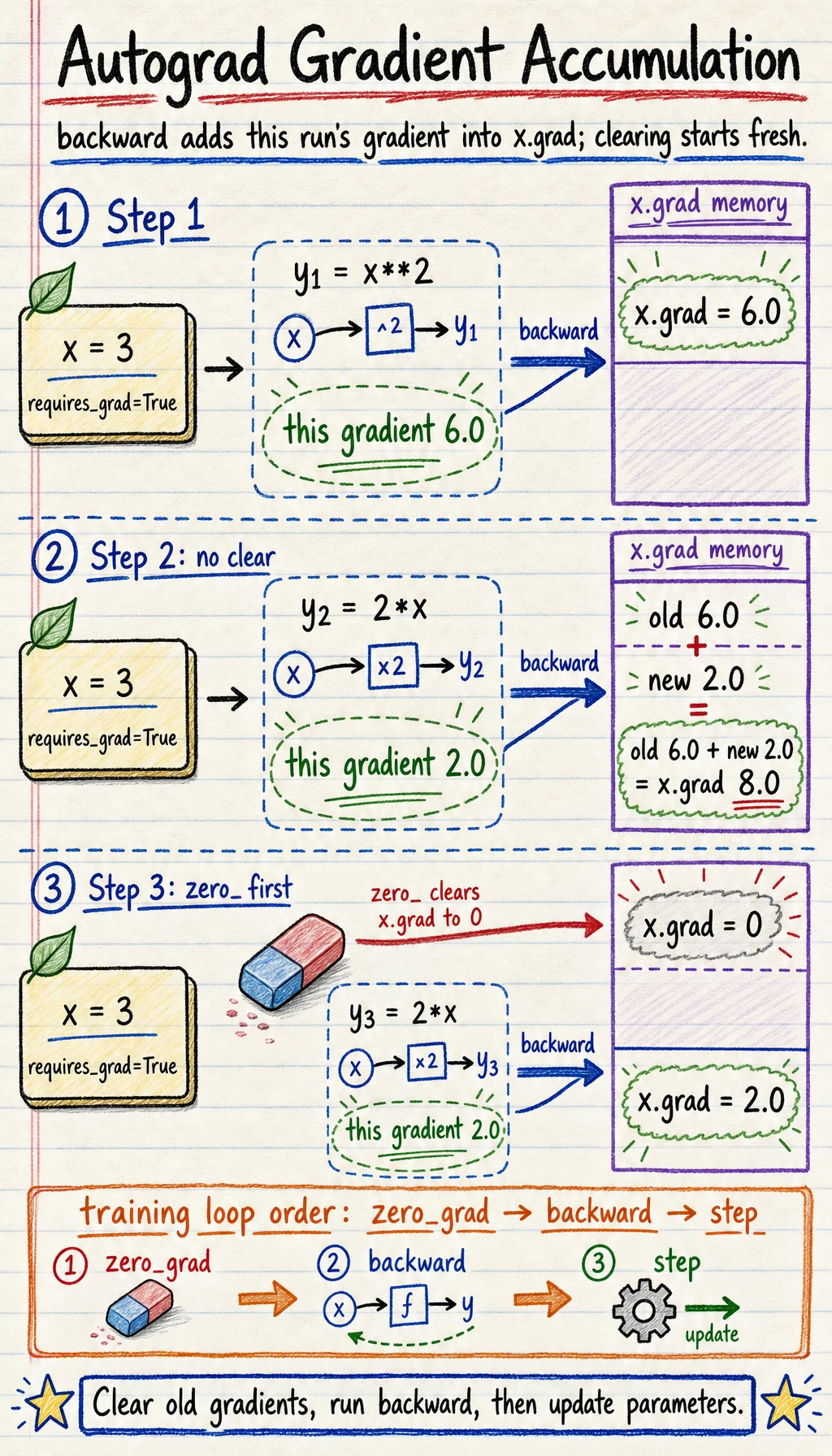
In normal training code, this is why each iteration uses:

optimizer.zero_grad()
loss.backward()
optimizer.step()

Lab 4: Fit Two Parameters by Hand

Now train a tiny linear model without nn.Linear or an optimizer. This makes the learning loop completely visible.

import torch

# Target rule: y = 2x + 1
x = torch.tensor([1.0, 2.0, 3.0, 4.0])
y_true = torch.tensor([3.0, 5.0, 7.0, 9.0])

w = torch.tensor(0.0, requires_grad=True)
b = torch.tensor(0.0, requires_grad=True)
lr = 0.05

print("two_parameter_fit")
for epoch in range(201):
    y_pred = w * x + b
    loss = ((y_pred - y_true) ** 2).mean()

    loss.backward()

    with torch.no_grad():
        w -= lr * w.grad
        b -= lr * b.grad

    if epoch % 50 == 0:
        print(
            f"epoch={epoch:3d} "
            f"loss={loss.item():.4f} "
            f"w={w.item():.4f} "
            f"b={b.item():.4f}"
        )

    w.grad.zero_()
    b.grad.zero_()

Expected output:

two_parameter_fit
epoch=  0 loss=41.0000 w=1.7500 b=0.6000
epoch= 50 loss=0.0030 w=2.0452 b=0.8672
epoch=100 loss=0.0007 w=2.0212 b=0.9375
epoch=150 loss=0.0001 w=2.0100 b=0.9706
epoch=200 loss=0.0000 w=2.0047 b=0.9862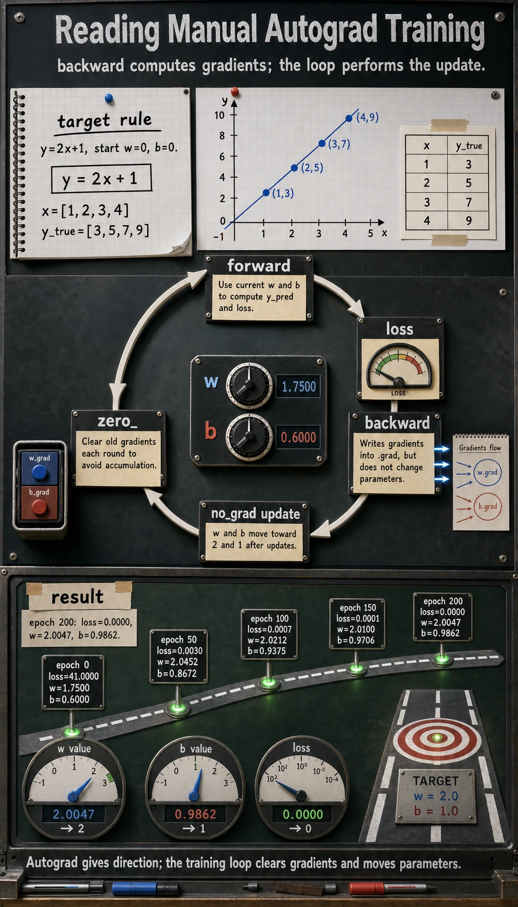

The parameters move toward w=2 and b=1. This is the same loop a neural network uses, only with millions of parameters instead of two.

requires_grad, no_grad, and detach

These three are related but not interchangeable.

Tool	Use it when	Effect
requires_grad=True	a tensor is a parameter or you need gradients for it	future operations are tracked
torch.no_grad()	inference or manual parameter update	temporarily stops graph recording
tensor.detach()	you want a tensor value without its graph history	returns a tensor disconnected from autograd

Runnable check:

import torch

w = torch.tensor(5.0, requires_grad=True)

tracked = w * 2
detached = tracked.detach()

with torch.no_grad():
    untracked = w * 3

print("tracked.requires_grad:", tracked.requires_grad)
print("detached.requires_grad:", detached.requires_grad)
print("untracked.requires_grad:", untracked.requires_grad)

Expected output:

tracked.requires_grad: True
detached.requires_grad: False
untracked.requires_grad: False

Practical examples:

• Use no_grad() during validation and prediction.
• Use detach() before logging tensors, converting to NumPy, or storing values that should not keep the whole graph alive.
• Do not detach tensors that still need to contribute gradients to the loss.

Common Error Patterns

Symptom	Likely cause	Fix
.grad is None	tensor does not require gradients, or it is not a leaf tensor	check requires_grad, inspect model parameters
training becomes unstable	gradients were not cleared	call optimizer.zero_grad() before backward()
RuntimeError: Trying to backward through the graph a second time	reused a graph after backward	recompute the forward pass, or use retain_graph=True only when you know why
memory keeps growing	storing graph-connected tensors in a list	store loss.item() or tensor.detach()
validation is slow and memory-heavy	gradients are tracked during evaluation	wrap validation in with torch.no_grad():

Use retain_graph=True Carefully

Most beginner code should not need retain_graph=True. If you reach for it, first ask: “Am I accidentally calling backward() twice on the same forward result instead of recomputing the forward pass?”

Quick Debug Checklist

Before backward():

print("loss requires_grad:", loss.requires_grad)
print("w requires_grad:", w.requires_grad)

After backward():

print("w.grad:", w.grad)
print("b.grad:", b.grad)

In a normal training loop, the order is:

forward→loss→zero_grad→backward→step

Some code uses zero_grad before forward, but the key rule is the same: clear old gradients before the next update.

Evidence to Keep

Keep one autograd trace:

Loss Requires Grad

True

Parameter Requires Grad

True

Grad After Backward

not None

Update Rule

backward computes gradients, optimizer or manual code updates values

Safe Logging

store loss.item() or tensor.detach()

This prevents the most common misconception: backward() is not the update. It only fills gradients.

Exercises

1. Change Lab 4 to learn y = 3x - 2. What should w and b approach?
2. Remove w.grad.zero_() and b.grad.zero_() in Lab 4. What happens?
3. Change lr to 0.5 and 0.005. Which one is unstable, and which one is slow?
4. Store loss itself in a list for 200 epochs, then store loss.item() instead. Why is the second safer?

Reference implementation and walkthrough

1. w should move toward 3, and b should move toward -2. Small differences are normal if the data has noise or training stops early.
2. Gradients accumulate by default. Without zero_(), each update mixes the current gradient with previous gradients, so the step size effectively becomes wrong and training can become unstable.
3. lr=0.5 is more likely to overshoot or diverge. lr=0.005 is usually slow because every update is tiny.
4. Saving loss tensors can keep references to computation graphs and waste memory. loss.item() stores only the Python number, which is safer for logging.

Key Takeaways

• Autograd records the computation graph from parameters to loss.
• backward() computes gradients; it does not update parameters.
• Gradients accumulate by default, so clear them before the next update.
• Use no_grad() for inference and manual updates; use detach() when you need a value without graph history.