5.6.2 Project 1: House Price Prediction (Regression Problem)

Project Positioning

This is your first complete ML regression project. You will go through the full workflow, from data exploration to model deployment. We use the built-in California Housing dataset from sklearn.

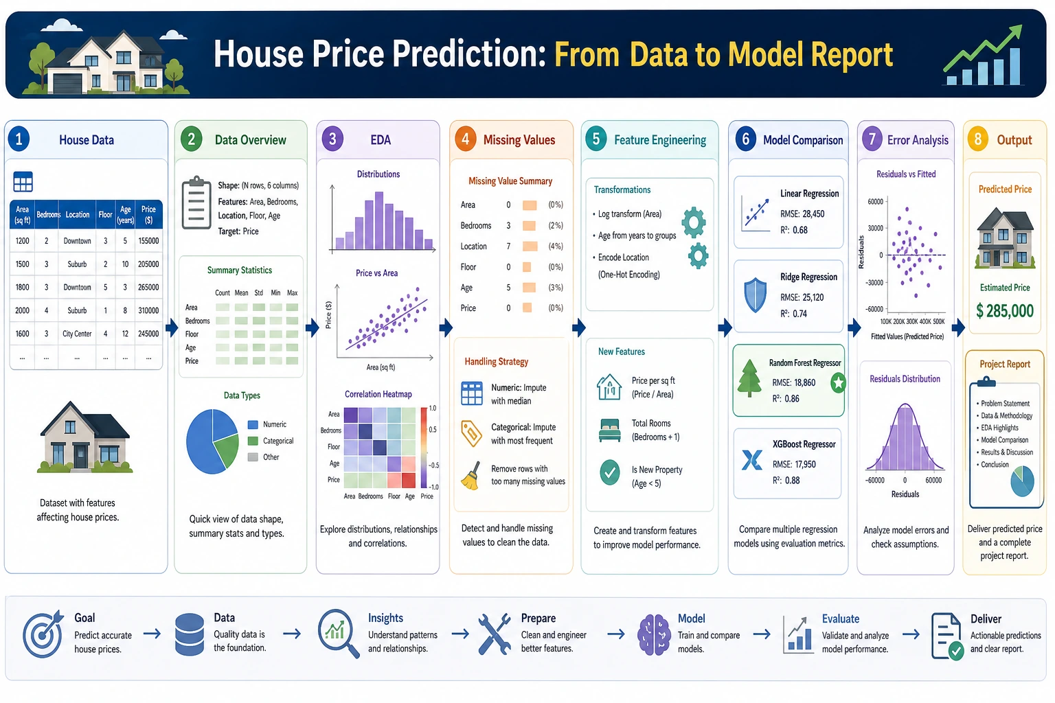
Project Overview

Info	Description
Task type	Regression
Dataset	California Housing (built into sklearn)
Evaluation metrics	RMSE, R²
Skills involved	EDA, feature engineering, multi-model comparison, tuning

Key Terms Before You Read the Code

• EDA (Exploratory Data Analysis) means looking at distributions, missing values, outliers, and correlations before modeling. In this project, EDA tells us what kind of price distribution we are trying to predict.
• RMSE (Root Mean Squared Error) measures the average prediction error in the same unit as the target. Smaller is better, and large mistakes are punished more heavily.
• R² (coefficient of determination) tells us how much variation in the target the model explains. Closer to 1 is better, but it should always be read together with RMSE.
• GBDT (Gradient Boosting Decision Tree) is a tree-based ensemble method that builds many small trees one after another, with each new tree trying to fix previous errors.

Running note

fetch_california_housing() may download the dataset the first time you run it, then cache it locally. If your environment is offline, run this once with network access first, or replace it with a local CSV that has similar numeric housing features.

---

First, Build a Map

This project is especially good for practicing “what should a regression project actually look like?”

flowchart LR
    A["Look at the data and target distribution"] --> B["Start with a linear regression baseline"]
    B --> C["Do a small amount of feature engineering"]
    C --> D["Compare tree models / GBDT"]
    D --> E["Tune hyperparameters"]
    E --> F["Residual analysis and interpretation"]

    style A fill:#e3f2fd,stroke:#1565c0,color:#333
    style F fill:#e8f5e9,stroke:#2e7d32,color:#333

A Better Beginner-Friendly Analogy

You can think of the house price prediction project like this:

• First estimate a batch of houses, then go back and see where your estimates were off

This is very similar to many real business scenarios:

• It’s not enough to output just a number
• You also need to know why that number is roughly reasonable
• And where you are most likely to make mistakes

If this is your first regression project, follow this path. It is usually the most stable.

What You’re Really Practicing Here

This project is not just about “making a regression model run.” More importantly, you are practicing these 4 things:

1. Finding useful clues from data exploration
2. Setting up a simple baseline first
3. Improving performance through feature engineering and model comparison
4. Explaining where the model does well and where it does poorly through error analysis

Why Is This Project Especially Good as Your First Complete Project?

Because it has several advantages:

• The task is simple and clear: regression
• The metrics are intuitive, and RMSE and R² are easy to explain
• The baseline is easy to establish
• There is a clear path for improvement later

Recommended Order

A better order for beginners is usually:

1. Start with the simplest linear regression baseline
2. Then do basic feature engineering
3. Then try tree models or GBDT
4. Only then do hyperparameter tuning

If you jump straight to complex models at the beginning, you will often lose your feel for the problem itself.

The Most Important Goal in the First Version Is Not a High Score

For the first version, there are really only two main goals:

1. Confirm that this problem can be modeled with regression
2. Build a baseline that all future improvements can be compared against

In other words, a first version that is “simple but complete” is more valuable than one that is “complex but hard to explain.”

Step 1: Load and Explore the Data

import pandas as pd
import numpy as np
import matplotlib.pyplot as plt
import seaborn as sns
from sklearn.datasets import fetch_california_housing

# Load data
data = fetch_california_housing()
df = pd.DataFrame(data.data, columns=data.feature_names)
df['MedHouseVal'] = data.target  # Median house value (in $100,000s)

print(f"Data shape: {df.shape}")
print(df.describe())

# Target distribution
fig, axes = plt.subplots(1, 2, figsize=(12, 4))
df['MedHouseVal'].hist(bins=50, ax=axes[0], color='steelblue', edgecolor='white')
axes[0].set_title('House Price Distribution')
axes[0].set_xlabel('Median house value (in $100,000s)')

# Correlation
corr = df.corr()['MedHouseVal'].drop('MedHouseVal').sort_values()
corr.plot.barh(ax=axes[1], color='coral')
axes[1].set_title('Correlation Between Features and House Price')
plt.tight_layout()
plt.show()

Step 1.1 What Should You Ask Most at This Stage

When you first look at the data, don’t rush to make charts. First ask these questions:

• Is the target distribution skewed?
• Are there any obvious outlier ranges?
• Which features may be strongly correlated with price?
• Which features are likely to be only weak signals?

These questions will directly affect:

• What baseline to start with
• Which feature engineering steps to prioritize
• Which dimensions to inspect in error analysis

Step 1.2 A Useful Beginner Rule to Remember

A very common mistake in first regression projects is:

• Rushing to change models immediately

A more stable order is usually:

• Look at the data first
• Understand the target
• Know what kind of distribution you are predicting

---

Step 2: Feature Engineering

# Create new features
df['rooms_per_household'] = df['AveRooms'] / df['AveOccup']
df['bedrooms_ratio'] = df['AveBedrms'] / df['AveRooms']
df['population_per_household'] = df['Population'] / df['HouseAge']

# Prepare data
from sklearn.model_selection import train_test_split

feature_cols = [c for c in df.columns if c != 'MedHouseVal']
X = df[feature_cols]
y = df['MedHouseVal']
X_train, X_test, y_train, y_test = train_test_split(X, y, test_size=0.2, random_state=42)
print(f"Training set: {X_train.shape}, Test set: {X_test.shape}")

Step 2.1 Why You Should Be Conservative the First Time You Do Feature Engineering

One of the most common mistakes in regression projects is adding too many features at once, and then not being able to tell which ones actually helped. A more stable approach is:

• Add only 2–3 new features with strong interpretability first
• Compare against the baseline every time you add something
• If there is no clear gain, don’t keep it just because it “looks advanced”

Step 2.2 A Feature Idea That Looks More Like Real Business Work

In house price problems, useful features are often related to “unit cost” and “relative position,” such as:

• Rooms per household
• Population per household
• Combinations of house age and location

These are more like real modeling thinking than just mechanically stacking more columns.

---

Step 3: Compare Multiple Models

from sklearn.linear_model import LinearRegression, Ridge
from sklearn.ensemble import RandomForestRegressor, GradientBoostingRegressor
from sklearn.preprocessing import StandardScaler
from sklearn.pipeline import make_pipeline
from sklearn.metrics import mean_squared_error, r2_score

models = {
    'Linear Regression': make_pipeline(StandardScaler(), LinearRegression()),
    'Ridge': make_pipeline(StandardScaler(), Ridge(alpha=1.0)),
    'Random Forest': RandomForestRegressor(n_estimators=100, random_state=42),
    'GBDT': GradientBoostingRegressor(n_estimators=100, random_state=42),
}

results = {}
for name, model in models.items():
    model.fit(X_train, y_train)
    y_pred = model.predict(X_test)
    rmse = np.sqrt(mean_squared_error(y_test, y_pred))
    r2 = r2_score(y_test, y_pred)
    results[name] = {'RMSE': rmse, 'R²': r2}
    print(f"{name:10s} | RMSE: {rmse:.4f} | R²: {r2:.4f}")

# Visualization
fig, ax = plt.subplots(figsize=(8, 5))
names = list(results.keys())
r2s = [v['R²'] for v in results.values()]
bars = ax.bar(names, r2s, color=['steelblue', 'coral', 'seagreen', 'gold'], alpha=0.8)
for bar, score in zip(bars, r2s):
    ax.text(bar.get_x() + bar.get_width()/2, bar.get_height() + 0.005,
            f'{score:.4f}', ha='center')
ax.set_ylabel('R²')
ax.set_title('Model R² Comparison')
ax.grid(axis='y', alpha=0.3)
plt.show()

Step 3.1 What Should You Pay Attention to When Comparing Models

Don’t just look at which R² is the highest. A more reliable comparison is to look at all of these together:

• Did RMSE decrease significantly?
• Did model complexity increase a lot?
• Did interpretability become much worse?

When you do your first regression project, what is most worth valuing is not the “best score model,” but:

• You know why it is better than the baseline
• You know exactly how it is better

Step 3.2 A Model Comparison Table Beginners Can Copy Directly

Model	Advantages	First focus
Linear Regression	Easiest to explain	Is the baseline stable?
Ridge	Slightly more stable	Does regularization help?
Random Forest	Stronger nonlinearity	Feature importance and overfitting risk
GBDT	Often stronger performance	Does RMSE drop noticeably?

This table is great for beginners because it turns “model names” back into “why are we trying this?”

---

Step 4: Hyperparameter Tuning

from sklearn.model_selection import RandomizedSearchCV
from scipy.stats import randint, uniform

param_dist = {
    'n_estimators': randint(100, 500),
    'max_depth': randint(5, 20),
    'learning_rate': uniform(0.01, 0.2),
    'subsample': uniform(0.7, 0.3),
}

rs = RandomizedSearchCV(
    GradientBoostingRegressor(random_state=42),
    param_dist, n_iter=30, cv=5,
    scoring='neg_root_mean_squared_error',
    random_state=42, n_jobs=-1
)
rs.fit(X_train, y_train)

y_pred_best = rs.predict(X_test)
print(f"Tuned RMSE: {np.sqrt(mean_squared_error(y_test, y_pred_best)):.4f}")
print(f"Tuned R²: {r2_score(y_test, y_pred_best):.4f}")
print(f"Best parameters: {rs.best_params_}")

---

Step 5: Result Analysis

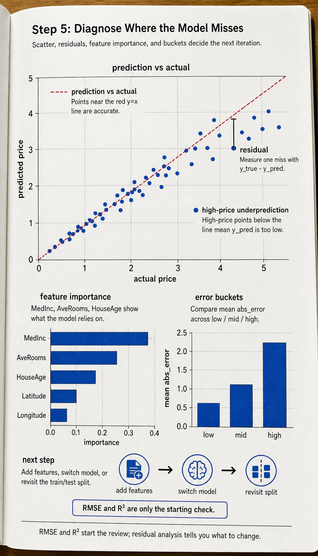
Read this map as a result checklist: first compare prediction vs actual, then inspect residual patterns before changing the model.

# Prediction vs actual
fig, axes = plt.subplots(1, 2, figsize=(12, 5))

axes[0].scatter(y_test, y_pred_best, s=5, alpha=0.3)
axes[0].plot([0, 5], [0, 5], 'r--')
axes[0].set_xlabel('Actual house price')
axes[0].set_ylabel('Predicted house price')
axes[0].set_title('Prediction vs Actual')

# Feature importance
importance = rs.best_estimator_.feature_importances_
sorted_idx = np.argsort(importance)
axes[1].barh(range(len(sorted_idx)), importance[sorted_idx], color='coral')
axes[1].set_yticks(range(len(sorted_idx)))
axes[1].set_yticklabels(np.array(feature_cols)[sorted_idx])
axes[1].set_title('Feature Importance')

plt.tight_layout()
plt.show()

Step 5.1 Residual Analysis Shows Your Project Skills Better Than the Final Score

A lot of people stop here at RMSE and R². But what really separates project quality is often residual analysis:

• Which price ranges have especially large errors?
• Does the model systematically underpredict high-priced homes?
• Which combinations of regional features are easiest to predict incorrectly?

This step directly tells you whether you should next:

• Add more features
• Switch models
• Or revisit the data split strategy

Step 5.2 Another Minimal Example of “Error Bucketing”

errors = pd.DataFrame({
    "y_true": [1.0, 2.5, 4.2, 3.8],
    "y_pred": [1.2, 2.0, 3.1, 4.5],
})
errors["abs_error"] = (errors["y_true"] - errors["y_pred"]).abs()
errors["bucket"] = pd.cut(errors["y_true"], bins=[0, 2, 4, 6], labels=["low", "mid", "high"])

print(errors.groupby("bucket", observed=False)["abs_error"].mean())

Expected output:

bucket
low     0.2
mid     0.6
high    1.1
Name: abs_error, dtype: float64

This example is very suitable for beginners because it helps you build one key habit first:

• Don’t only look at the overall average error
• Also look at which kinds of samples are easier to get wrong

In this tiny example, the high-price bucket has the largest average error. That does not prove every real house-price model will fail on high-price homes, but it shows exactly how Step 5 turns a scatter plot into an improvement question: which bucket should we investigate next?

---

A Very Beginner-Friendly Minimal Review Table

You can make a table like this directly:

Version	What changed	My judgment
baseline	Linear regression	Establish a lower bound first
v2	Added 2-3 features	See whether feature engineering really helps
v3	Switched to tree model / GBDT	See whether a nonlinear model fits better

Keep RMSE and R² in your notebook or experiment log. In the written project report, only show the metric columns after you have real values to compare.

This table turns your project from “code that ran” into “a project with a clear iteration process.”

A Project Checklist Worth Copying for Beginners

When you do a house price prediction project for the first time, the most stable checklist is usually:

1. Has the baseline been established?
2. Do the engineered features have clear business meaning?
3. Are you comparing models using more than one metric?
4. Has residual analysis already told you what to improve next?

If you have done all 4 of these well, then this project is no longer “just running a regression script,” but a real end-to-end modeling exercise.

If You Keep Improving This Project, What Is Most Worth Adding?

The most valuable additions are usually:

1. Residual distribution analysis
2. Error comparison across different regions / price ranges
3. A clear explanation of how the project evolved from baseline to best model

That makes the project feel more like a real modeling and review effort.

Evidence to Keep

Keep this page’s proof of learning as a small evidence card:

Project Goal

prediction, segmentation, Kaggle, or end-to-end ML portfolio target

Pipeline

data split, preprocessing, model, evaluation, and report artifacts

Result

metric table, chart, predictions, failure samples, and README note

Failure Check

non-reproducible run, leakage, overfitting, weak baseline, or missing deployment boundary

Expected Output

ML project folder with pipeline, metrics, and failure review

What You Should Include When Delivering the Project

• A chart of “actual values vs predicted values”
• A short explanation of error sources
• A comparison table between the baseline and the improved version
• A summary of “what I would improve next if I continued”

What Is Most Worth Showing in a Portfolio Version

If you want to turn this into a portfolio page, what matters most is not a long list of model names, but:

1. What your baseline was
2. Which improvement was the most effective
3. How RMSE / R² changed before and after
4. What you learned from residual analysis
5. What you plan to improve next

---

Project Checklist

• Complete EDA: distribution, correlation, missing values
• Feature engineering: create at least 2 new features
• Compare at least 3 models
• Tune hyperparameters for the best model
• Perform residual analysis and feature importance analysis

Project reference and review notes

1. EDA is complete only when distributions, missing values, correlations, and suspicious outliers are recorded with a short modeling implication.
2. Engineered features should have clear housing meaning, such as area ratios or quality aggregates. If a feature uses future or target-derived information, reject it as leakage.
3. Compare models with the same split or cross-validation setup. Include a plain baseline so the improved model has something honest to beat.
4. Hyperparameter tuning should happen after a working baseline. Use validation or cross-validation, and keep the test set for the final check.
5. Residual analysis should say where the model misses most, such as high-price homes or a region bucket. The next experiment should come from that observation.

Recommended Version Roadmap

Version	Goal	Delivery focus
Basic version	Run the minimal closed loop	Can input, process, and output, with one set of examples retained
Standard version	Build a presentable project	Add configuration, logging, error handling, README, and screenshots
Challenge version	Get close to portfolio quality	Add evaluation, comparison experiments, failed sample analysis, and a next-step roadmap

It is recommended to finish the basic version first. Don’t try to make it big and complete all at once. Every time you improve a version, write into the README: “What capability was added, how it was verified, and what problems remain.”